Introduction
Argoverse 2 is a collection of open-source autonomous driving data and high-definition (HD) maps from six U.S. cities: Austin, Detroit, Miami, Pittsburgh, Palo Alto, and Washington, D.C. This release builds upon the initial launch of Argoverse, which was among the first data releases of its kind to include HD maps for machine learning and computer vision research.
Argoverse 2 includes four open-source datasets:
- Argoverse 2 Sensor Dataset: contains 1,000 3D annotated scenarios with lidar, stereo imagery, and ring camera imagery. This dataset improves upon the Argoverse 1 3D Tracking dataset.
- Argoverse 2 Motion Forecasting Dataset: contains 250,000 scenarios with trajectory data for many object types. This dataset improves upon the Argoverse 1 Motion Forecasting Dataset.
- Argoverse 2 Lidar Dataset: contains 20,000 unannotated lidar sequences.
- Argoverse 2 Map Change Detection Dataset: contains 1,000 scenarios, 200 of which depict real-world HD map changes.
Argoverse 2 datasets share a common HD map format that is richer than the HD maps in Argoverse 1. Argoverse 2 datasets also share a common API, which allows users to easily access and visualize the data and maps.
Where was the data collected?
The data in Argoverse 2 comes from six U.S. cities with complex, unique driving environments: Miami, Austin, Washington DC, Pittsburgh, Palo Alto, and Detroit. We include recorded logs of sensor data, or “scenarios,” across different seasons, weather conditions, and times of day.
How was the data collected?
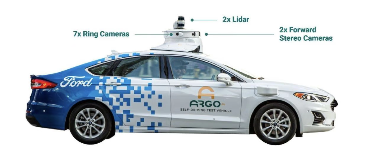
We collected all of our data using a fleet of identical Ford Fusion Hybrids, fully integrated with Argo AI self-driving technology. We include data from two lidar sensors, seven ring cameras, and two front-facing stereo cameras. All sensors are roof-mounted:
Lidar
- Two roof-mounted VLP-32C lidar sensors (64 beams total)
- Overlapping 40° vertical field of view
- Range of 200 m
- On average, our lidar sensors produce a point cloud with ~ 107,000 points at 10 Hz
Cameras
- Seven high-resolution ring cameras (2048 width x 1550 height) recording at 20 Hz with a combined 360° field of view. Unlike Argoverse 1, the camera and lidar are synchronized. The camera images are captured as one of the two lidars sweep past its field of view. The front center camera is portrait aspect ratio (1550 width x 2048 height) to improve the vertical field of view.
- Two front-view facing stereo cameras (2048 x 1550) sampled at 20 Hz
Localization
We use a city-specific coordinate system for vehicle localization. We include 6-DOF localization for each timestamp, from a combination of GPS-based and sensor-based localization methods.
Calibration
Sensor measurements for each driving session are stored in “scenarios.” For each scenario, we provide intrinsic and extrinsic calibration data for the lidar and all nine cameras.
Argoverse 2 Maps
Each scenario is paired with a local map. Our HD maps contain rich geometric and semantic metadata for better 3D scene understanding.
Vector Map: Lane-Level Geometry
Our semantic vector map contains 3D lane-level details, such as lane boundaries, lane marking types, traffic direction, crosswalks, driveable area polygons, and intersection annotations. These map attributes are powerful priors for perception and forecasting. For example, vehicle heading tends to follow lane direction, drivers are more likely to make lane changes where there are dashed lane boundaries, and pedestrians are more likely to cross the street at designated crosswalks.
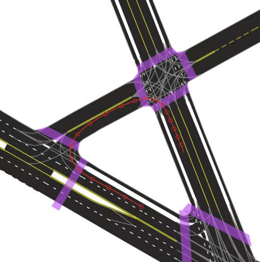
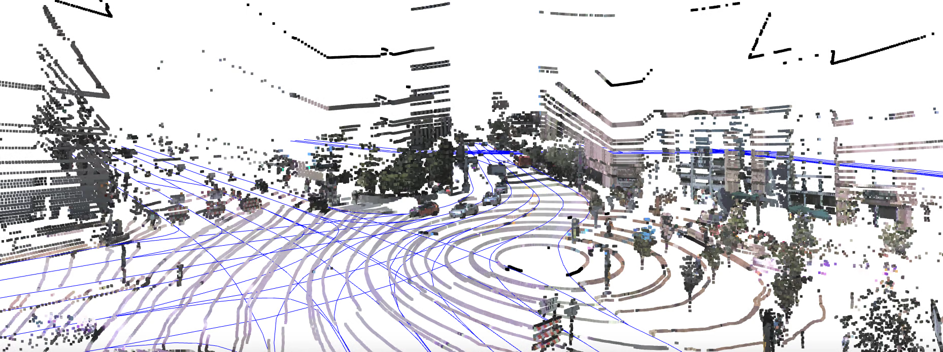
An example of an HD map for an Argoverse 2 scenario. This map format is shared by the Sensor, Lidar, Motion Forecasting, and Map Change datasets. This figure shows a rendering of the “vector” map with polygons and lines defining lanes, lane boundaries (dashed white, dashed yellow, double yellow, etc), and crosswalks (purple). Implicit lane boundaries, such as the corridor a vehicle is likely to follow through an intersection, are shown in gray. The path of the ego-vehicle is shown in red.
Raster Map: Ground Height
To support the Sensor and Map Change datasets, our maps include real-valued ground height at thirty centimeter resolution. With these map attributes, it is easy to filter out ground lidar returns (e.g. for object detection) or to keep only ground lidar returns (e.g. for building a bird’s-eye view rendering).

Ground height samples for an Argoverse 2 scenario. Ground height samples are visualized as blue points. Lidar samples are shown with color projected from ring camera imagery.
Getting Started
If you would like to take advantage of the most recent features, please install via conda/install.sh.
Table of Contents
Overview
This section covers the following:
- Installing
av2. - Downloading the Argoverse 2 and TbV datasets.
Setup
We highly recommend using conda with the conda-forge channel for package management.
Installing via conda (recommended)
You will need to install conda on your machine. We recommend installing miniforge:
wget -O Miniforge3.sh "https://github.com/conda-forge/miniforge/releases/latest/download/Miniforge3-$(uname)-$(uname -m).sh"
bash Miniforge3.sh -bp "${HOME}/conda"
Then, install av2:
bash conda/install.sh && conda activate av2
You may need to run a post-install step to initialize conda:
$(which conda) init $SHELL
If conda is not found, you will need to add the binary to your PATH environment variable.
Installing via pip
Installation via PyPI requires manually installing Rust via rustup.
Run the following and select the default installation:
curl --proto '=https' --tlsv1.2 -sSf https://sh.rustup.rs | sh
Make sure to adjust your PATH as:
export PATH=$HOME/.cargo/bin:$PATH
We use the nightly release of Rust for SIMD support. Set it as your default toolchain:
rustup default nightly
Then, install av2:
pip install git+https://github.com/argoverse/av2-api#egg=av2
Downloading the data
Our datasets are available for download from AWS S3.
For the best experience, we highly recommend using the open-source s5cmd tool to transfer the data to your local filesystem. Please note that an AWS account is not required to download the datasets.
Additional info can be found at https://aws.amazon.com/blogs/opensource/parallelizing-s3-workloads-s5cmd/.
Installing s5cmd
Conda Installation (Recommended)
The easiest way to install s5cmd is through conda using the conda-forge channel:
conda install s5cmd -c conda-forge
Manual Installation
s5cmd can also be installed with the following script:
#!/usr/bin/env bash

export INSTALL_DIR=$HOME/.local/bin
export PATH=$PATH:$INSTALL_DIR
export S5CMD_URI=https://github.com/peak/s5cmd/releases/download/v2.0.0/s5cmd_2.0.0_$(uname | sed 's/Darwin/macOS/g')-64bit.tar.gz

mkdir -p $INSTALL_DIR
curl -sL $S5CMD_URI | tar -C $INSTALL_DIR -xvzf - s5cmd
Note that it will install s5cmd in your local bin directory. You can always change the path if you prefer installing it in another directory.
Download the Datasets
Run the following command to download the one or more of the datasets:
#!/usr/bin/env bash

# Dataset URIs
# s3://argoverse/datasets/av2/sensor/
# s3://argoverse/datasets/av2/lidar/
# s3://argoverse/datasets/av2/motion-forecasting/
# s3://argoverse/datasets/av2/tbv/

export DATASET_NAME="sensor"  # sensor, lidar, motion_forecasting or tbv.
export TARGET_DIR="$HOME/data/datasets"  # Target directory on your machine.

s5cmd --no-sign-request cp "s3://argoverse/datasets/av2/$DATASET_NAME/*" $TARGET_DIR
The command will all data for $DATASET_NAME to $TARGET_DIR. Given the size of the dataset, it might take a couple of hours depending on the network connectivity.
When the download is finished, the dataset is ready to use!
FAQ
Why manage dependencies in
condainstead ofpip?
conda enables package management outside of the python ecosystem. This enables us to specify all necessary dependencies in environment.yml. Further, gpu-based packages (e.g., torch) are handled better through conda.
Why
conda-forge?
conda-forge is a community-driven channel of conda recipes. It includes a large number of packages which can all be properly tracked in the conda resolver allowing for consistent environments without conflicts.
Datasets
The Argoverse 2 API supports multiple datasets spanning two separate publications.
-
- Sensor
- Lidar
- Motion Forecasting
-
- Map Change Detection
Sensor Dataset
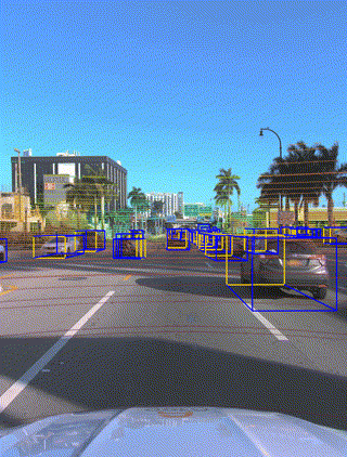
Table of Contents
- Overview
- Sensor Suite
- Dataset Structure Format
- Annotations
- Pose
- LiDAR Sweeps
- Calibration
- Intrinsics
- Log Distribution Across Cities
- Privacy
- Sensor Dataset splits
- Sensor Dataset Taxonomy
Overview
The Argoverse 2 Sensor Dataset is the successor to the Argoverse 1 3D Tracking Dataset. AV2 is larger, with 1,000 scenes totalling 4.2 hours of driving data, up from 113 scenes in Argoverse 1.
The total dataset amounts to 1 TB of data in its extracted form. Each vehicle log is approximately 15 seconds in duration and 1 GB in size, including ~150 LiDAR sweeps on average, and ~300 images from each of the 9 cameras (~2700 images per log).
Sensor Suite
Lidar sweeps are collected at 10 Hz, along with 20 fps imagery from 7 ring cameras positioned to provide a fully panoramic field of view, and 20 fps imagery from 2 stereo cameras. In addition, camera intrinsics, extrinsics and 6-DOF ego-vehicle pose in a global coordinate system are provided. Lidar returns are captured by two 32-beam lidars, spinning at 10 Hz in the same direction, but separated in orientation by 180°. The cameras trigger in-sync with both lidars, leading to a 20 Hz frame-rate. The nine global shutter cameras are synchronized to the lidar to have their exposure centered on the lidar sweeping through their fields of view.
We aggregate all returns from the two stacked 32-beam sensors into a single sweep. These sensors each have different, overlapping fields-of-view. Both lidars have their own reference frame, and we refer to them as up_lidar and down_lidar, respectively. We have egomotion-compensated the LiDAR sensor data to the egovehicle reference nanosecond timestamp. All LiDAR returns are provided in the egovehicle reference frame, not the individual LiDAR reference frame.
Imagery is provided at (height x width) of 2048 x 1550 (portrait orientation) for the ring front-center camera, and at 1550 x 2048 (landscape orientation) for all other 8 cameras (including the stereo cameras). All camera imagery is provided in an undistorted format.

Dataset Structure Format
Tabular data (annotations, lidar sweeps, poses, calibration) are provided as Apache Feather Files with the file extension .feather. We show examples below.
Annotations
Object annotations are provided as 3d cuboids. Their pose is provided in the egovehicle’s reference frame.
io_utils.read_feather("{AV2_ROOT}/01bb304d-7bd8-35f8-bbef-7086b688e35e/annotations.feather")
             timestamp_ns  track_uuid          category  length_m   width_m  height_m    qw   qx   qy    qz    tx_m   ty_m  tz_m  num_interior_pts
0      315968867659956000 022c398c...           BOLLARD  0.363046  0.222484  0.746710  0.68  0.0  0.0  0.72   25.04  -2.55  0.01                10
1      315968867659956000 12361d61...           BOLLARD  0.407004  0.206964  0.792624  0.68  0.0  0.0  0.72   34.13  -2.51 -0.05                 5
2      315968867659956000 12cac1ed...           BOLLARD  0.337859  0.227949  0.747096  0.70  0.0  0.0  0.71   21.99  -2.55  0.03                13
3      315968867659956000 173910b2...           BOLLARD  0.326865  0.204709  0.809859  0.71  0.0  0.0  0.69    3.79  -2.53  0.05                16
4      315968867659956000 23716fb2...           BOLLARD  0.336697  0.226178  0.820867  0.72  0.0  0.0  0.69    6.78  -2.52  0.04                19
...                   ...         ...               ...       ...       ...       ...   ...  ...  ...   ...     ...    ...   ...               ...
18039  315968883159714000 c48fc856...          STROLLER  0.581798  0.502284  0.991001  0.97  0.0  0.0 -0.22  -10.84  34.33  0.14                13
18040  315968883159714000 cf1c4301...             TRUCK  9.500000  3.010952  3.573860 -0.51  0.0  0.0  0.85  -26.97   0.09  1.41              1130
18041  315968883159714000 a834bc72...         TRUCK_CAB  9.359874  3.260000  4.949222  0.51  0.0  0.0  0.85  138.13  13.39  0.80                18
18042  315968883159714000 ff50196f... VEHICULAR_TRAILER  3.414590  2.658412  2.583414  0.84  0.0  0.0  0.52  -13.95   8.32  1.28               533
18043  315968883159714000 a748a5c4...    WHEELED_DEVICE  1.078700  0.479100  1.215600  0.72  0.0  0.0  0.69   19.17  -6.07  0.28                 7
Pose
6-DOF ego-vehicle pose in a global (city) coordinate system is provided (visualized in the figure below as a red line, with red circles indicated at a 1 Hz frequency):

We refer to this pose as city_SE3_egovehicle throughout the codebase:
>>> io_utils.read_feather("{AV2_ROOT}/54bc6dbc-ebfb-3fba-b5b3-57f88b4b79ca/city_SE3_egovehicle.feather")
            timestamp_ns        qw        qx        qy        qz        tx_m         ty_m       tz_m
0     315968112437425433 -0.740565 -0.005635 -0.006869 -0.671926  747.405602  1275.325609 -24.255610
1     315968112442441182 -0.740385 -0.005626 -0.006911 -0.672124  747.411245  1275.385425 -24.255906
2     315968112449927216 -0.740167 -0.005545 -0.006873 -0.672365  747.419676  1275.474686 -24.256406
3     315968112449927217 -0.740167 -0.005545 -0.006873 -0.672365  747.419676  1275.474686 -24.256406
4     315968112457428271 -0.739890 -0.005492 -0.006953 -0.672669  747.428448  1275.567576 -24.258680
...                  ...       ...       ...       ...       ...         ...          ...        ...
2692  315968128362451249 -0.694376 -0.001914 -0.006371 -0.719582  740.163738  1467.061503 -24.546971
2693  315968128372412943 -0.694326 -0.001983 -0.006233 -0.719631  740.160489  1467.147020 -24.545918
2694  315968128377482496 -0.694346 -0.001896 -0.006104 -0.719613  740.158684  1467.192399 -24.546316
2695  315968128387425439 -0.694307 -0.001763 -0.005998 -0.719652  740.155543  1467.286735 -24.549918
2696  315968128392441187 -0.694287 -0.001728 -0.005945 -0.719672  740.153742  1467.331549 -24.550363

[2697 rows x 8 columns]
LiDAR Sweeps
For example, we show below the format of an example sweep sensors/lidar/15970913559644000.feather (the sweep has a reference timestamp of 15970913559644000 nanoseconds):
               x          y         z  intensity  laser_number  offset_ns
0      -1.291016   2.992188 -0.229370         24            31    3318000
1     -25.921875  25.171875  0.992188          5            14    3318000
2     -15.500000  18.937500  0.901855         34            16    3320303
3      -3.140625   4.593750 -0.163696         12            30    3320303
4      -4.445312   6.535156 -0.109802         14            29    3322607
...          ...        ...       ...        ...           ...        ...
98231  18.312500 -38.187500  3.279297         26            50  106985185
98232  23.109375 -34.437500  3.003906         20            49  106987490
98233   4.941406  -5.777344 -0.162720         12            32  106987490
98234   6.640625  -8.257812 -0.157593          6            33  106989794
98235  20.015625 -37.062500  2.550781         12            47  106989794

[98236 rows x 6 columns]
Calibration
An example calibration file is shown below, parameterizing vehicle_SE3_sensor for each sensor (the sensor’s pose in the egovehicle coordinate system):
>>> io_utils.read_feather(f"{AV2_ROOT}/54bc6dbc-ebfb-3fba-b5b3-57f88b4b79ca/calibration/egovehicle_SE3_sensor.feather")
           sensor_name        qw        qx        qy        qz      tx_m      ty_m      tz_m
0    ring_front_center  0.502809 -0.499689  0.500147 -0.497340  1.631216 -0.000779  1.432780
1      ring_front_left  0.635526 -0.671957  0.275463 -0.262107  1.550015  0.197539  1.431329
2     ring_front_right  0.264354 -0.278344  0.671740 -0.633567  1.554057 -0.194171  1.430575
3       ring_rear_left  0.600598 -0.603227 -0.371096  0.371061  1.104117  0.124369  1.446070
4      ring_rear_right -0.368149  0.369885  0.603626 -0.602733  1.103432 -0.128317  1.428135
5       ring_side_left  0.684152 -0.724938 -0.058345  0.054735  1.310427  0.267904  1.433233
6      ring_side_right -0.053810  0.056105  0.727113 -0.682103  1.310236 -0.273345  1.435529
7    stereo_front_left  0.500421 -0.499934  0.501241 -0.498399  1.625085  0.248148  1.222831
8   stereo_front_right  0.500885 -0.503584  0.498793 -0.496713  1.633076 -0.250872  1.222173
9             up_lidar  0.999996  0.000000  0.000000 -0.002848  1.350180  0.000000  1.640420
10          down_lidar -0.000089 -0.994497  0.104767  0.000243  1.355162  0.000133  1.565252
Intrinsics
An example camera intrinsics file is shown below:
>>> io_utils.read_feather("{AV2_ROOT}/54bc6dbc-ebfb-3fba-b5b3-57f88b4b79ca/calibration/intrinsics.feather")
          sensor_name        fx_px        fy_px        cx_px  ...        k2        k3  height_px  width_px
0   ring_front_center  1773.504272  1773.504272   775.826693  ... -0.212167  0.328694       2048      1550
1     ring_front_left  1682.010713  1682.010713  1025.068254  ... -0.136984  0.209330       1550      2048
2    ring_front_right  1684.834479  1684.834479  1024.373455  ... -0.133341  0.208709       1550      2048
3      ring_rear_left  1686.494558  1686.494558  1025.655905  ... -0.129761  0.202326       1550      2048
4     ring_rear_right  1683.375120  1683.375120  1024.381124  ... -0.129331  0.201599       1550      2048
5      ring_side_left  1684.902403  1684.902403  1027.822264  ... -0.124561  0.196519       1550      2048
6     ring_side_right  1682.936559  1682.936559  1024.948976  ... -0.109515  0.179383       1550      2048
7   stereo_front_left  1685.825885  1685.825885  1025.830335  ... -0.113065  0.182441       1550      2048
8  stereo_front_right  1683.137591  1683.137591  1024.612074  ... -0.127301  0.198538       1550      2048
A local map is provided per log, please refer to the Map README for additional details.
Log Distribution Across Cities
Vehicle logs from the AV2 Sensor Dataset are captured in 6 cities, according to the following distribution:
- Austin, Texas: 31 logs.
- Detroit, Michigan: 117 logs.
- Miami, Florida: 354 logs.
- Pittsburgh, Pennsylvania: 350 logs.
- Palo Alto, California: 22 logs.
- Washington, D.C.: 126 logs.
Privacy
All faces and license plates, whether inside vehicles or outside of the drivable area, are blurred extensively to preserve privacy.
Sensor Dataset splits
We randomly partitioned 1000 logs into the following splits:
- Train (700 logs)
- Validation (150 logs)
- Test (150 logs)
Sensor Dataset Taxonomy
The AV2 Sensor Dataset contains 10 Hz 3D cuboid annotations for objects within our 30 class taxonomy. Objects are annotated if they are within the “region of interest” (ROI) – within five meters of the mapped “driveable” area.

These 30 classes are defined as follows, appearing in order of frequency:
-
REGULAR_VEHICLE: Any conventionally sized passenger vehicle used for the transportation of people and cargo. This includes Cars, vans, pickup trucks, SUVs, etc. -
PEDESTRIAN: Person that is not driving or riding in/on a vehicle. They can be walking, standing, sitting, prone, etc. -
BOLLARD: Bollards are short, sturdy posts installed in the roadway or sidewalk to control the flow of traffic. These may be temporary or permanent and are sometimes decorative. -
CONSTRUCTION_CONE: Movable traffic cone that is used to alert drivers to a hazard. These will typically be orange and white striped and may or may not have a blinking light attached to the top. -
CONSTRUCTION_BARREL: Construction Barrel is a movable traffic barrel that is used to alert drivers to a hazard. These will typically be orange and white striped and may or may not have a blinking light attached to the top. -
STOP_SIGN: Red octagonal traffic sign displaying the word STOP used to notify drivers that they must come to a complete stop and make sure no other road users are coming before proceeding. -
BICYCLE: Non-motorized vehicle that typically has two wheels and is propelled by human power pushing pedals in a circular motion. -
LARGE_VEHICLE: Large motorized vehicles (four wheels or more) which do not fit into any more specific subclass. Examples include extended passenger vans, fire trucks, RVs, etc. -
WHEELED_DEVICE: Objects involved in the transportation of a person and do not fit a more specific class. Examples range from skateboards, non-motorized scooters, segways, to golf-carts. -
BUS: Standard city buses designed to carry a large number of people. -
BOX_TRUCK: Chassis cab truck with an enclosed cube shaped cargo area. It should be noted that the cargo area is rigidly attached to the cab, and they do not articulate. -
SIGN: Official road signs placed by the Department of Transportation (DOT signs) which are of interest to us. This includes yield signs, speed limit signs, directional control signs, construction signs, and other signs that provide required traffic control information. Note that Stop Sign is captured separately and informative signs such as street signs, parking signs, bus stop signs, etc. are not included in this class. -
TRUCK: Vehicles that are clearly defined as a truck but does not fit into the subclasses of Box Truck or Truck Cab. Examples include common delivery vehicles (UPS, FedEx), mail trucks, garbage trucks, utility trucks, ambulances, dump trucks, etc. -
MOTORCYCLE: Motorized vehicle with two wheels where the rider straddles the engine. These are capable of high speeds similar to a car. -
BICYCLIST: Person actively riding a bicycle, non-pedaling passengers included. -
VEHICULAR_TRAILER: Non-motorized, wheeled vehicle towed behind a motorized vehicle. -
TRUCK_CAB: Heavy truck commonly known as “Semi cab”, “Tractor”, or “Lorry”. This refers to only the front of part of an articulated tractor trailer. -
MOTORCYCLIST: Person actively riding a motorcycle or a moped, including passengers. -
DOG: Any member of the canine family. -
SCHOOL_BUS: Bus that primarily holds school children (typically yellow) and can control the flow of traffic via the use of an articulating stop sign and loading/unloading flasher lights. -
WHEELED_RIDER: Person actively riding or being carried by a wheeled device. -
STROLLER: Push-cart with wheels meant to hold a baby or toddler. -
ARTICULATED_BUS: Articulated buses perform the same function as a standard city bus, but are able to bend (articulate) towards the center. These will also have a third set of wheels not present on a typical bus. -
MESSAGE_BOARD_TRAILER: Trailer carrying a large, mounted, electronic sign to display messages. Often found around construction sites or large events. -
MOBILE_PEDESTRIAN_SIGN: Movable sign designating an area where pedestrians may cross the road. -
WHEELCHAIR: Chair fitted with wheels for use as a means of transport by a person who is unable to walk as a result of illness, injury, or disability. This includes both motorized and non-motorized wheelchairs as well as low-speed seated scooters not intended for use on the roadway. -
RAILED_VEHICLE: Any vehicle that relies on rails to move. This applies to trains, trolleys, train engines, train freight cars, train tanker cars, subways, etc. -
OFFICIAL_SIGNALER: Person with authority specifically responsible for stopping and directing vehicles through traffic. -
TRAFFIC_LIGHT_TRAILER: Mounted, portable traffic light unit commonly used in construction zones or for other temporary detours. -
ANIMAL: All recognized animals large enough to affect traffic, but that do not fit into the Cat, Dog, or Horse categories
Argoverse 2 Lidar Dataset Overview
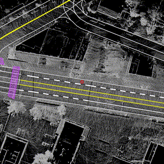


Table of Contents
Overview
The Argoverse 2 Lidar Dataset is intended to support research into self-supervised learning in the lidar domain as well as point cloud forecasting. The AV2 Lidar Dataset is mined with the same criteria as the Forecasting Dataset to ensure that each scene is interesting. While the Lidar Dataset does not have 3D object annotations, each scenario carries an HD map with rich, 3D information about the scene.
Dataset Size
Our dataset is the largest such collection to date with 20,000 thirty second sequences.
Sensor Suite
Lidar sweeps are collected at 10 Hz. In addition, 6-DOF ego-vehicle pose in a global coordinate system are provided. Lidar returns are captured by two 32-beam lidars, spinning at 10 Hz in the same direction, but separated in orientation by 180°.
We aggregate all returns from the two stacked 32-beam sensors into a single sweep. These sensors each have different, overlapping fields-of-view. Both lidars have their own reference frame, and we refer to them as up_lidar and down_lidar, respectively. We have egomotion-compensated the lidar sensor data to the egovehicle reference nanosecond timestamp. All lidar returns are provided in the egovehicle reference frame, not the individual lidar reference frame.
Dataset Structure Format
Tabular data (lidar sweeps, poses) are provided as Apache Feather Files with the file extension .feather.
Maps: A local vector map is provided per log, please refer to the Map README for additional details.
Directory structure:
av2
└───lidar
    └───train
    |   └───LyIXwbWeHWPHYUZjD1JPdXcvvtYumCWG
    |       └───sensors
    |       |   └───lidar
    |       |       └───15970913559644000.feather
    |       |                      .
    |       |                      .
    |       |                      .
    |       └───calibration
    |       |   └───egovehicle_SE3_sensor.feather
    |       └───map
    |       |   └───log_map_archive_LyIXwbWeHWPHYUZjD1JPdXcvvtYumCWG__Summer____PIT_city_77257.json
    |       └───city_SE3_egovehicle.feather
    └───val
    └───test
An example sweep sensors/lidar/15970913559644000.feather, meaning a reference timestamp of 15970913559644000 nanoseconds:
               x          y         z  intensity  laser_number  offset_ns
0      -1.291016   2.992188 -0.229370         24            31    3318000
1     -25.921875  25.171875  0.992188          5            14    3318000
2     -15.500000  18.937500  0.901855         34            16    3320303
3      -3.140625   4.593750 -0.163696         12            30    3320303
4      -4.445312   6.535156 -0.109802         14            29    3322607
...          ...        ...       ...        ...           ...        ...
98231  18.312500 -38.187500  3.279297         26            50  106985185
98232  23.109375 -34.437500  3.003906         20            49  106987490
98233   4.941406  -5.777344 -0.162720         12            32  106987490
98234   6.640625  -8.257812 -0.157593          6            33  106989794
98235  20.015625 -37.062500  2.550781         12            47  106989794

[98236 rows x 6 columns]
Lidar Dataset splits
We randomly partition the dataset into the following splits:
- Train (16,000 logs)
- Validation (2,000 logs)
- Test (2,000 logs)
Overview


Table of Contents
Overview
The Argoverse 2 motion forecasting dataset consists of 250,000 scenarios, collected from 6 cities spanning multiple seasons.
Each scenario is specifically designed to maximize interactions relevant to the ego-vehicle. This naturally results in the inclusion of actor-dense scenes featuring a range of vehicle and non-vehicle actor types. At the time of release, AV2 provides the largest object taxonomy, in addition to the broadest mapped area of any motion forecasting dataset released so far.
Download
The latest version of the AV2 motion forecasting dataset can be downloaded from the Argoverse website.
Scenarios and Tracks
Each scenario is 11s long and consists of a collection of actor histories, which are represented as “tracks”. For each scenario, we provide the following high-level attributes:
scenario_id: Unique ID associated with this scenario.timestamps_ns: All timestamps associated with this scenario.tracks: All tracks associated with this scenario.focal_track_id: The track ID associated with the focal agent of the scenario.city_name: The name of the city associated with this scenario.
Each track is further associated with the following attributes:
track_id: Unique ID associated with this trackobject_states: States for each timestep where the track object had a valid observation.object_type: Inferred type for the track object.category: Assigned category for track - used as an indicator for prediction requirements and data quality.
Track object states bundle all information associated with a particular actor at a fixed point in time:
observed: Boolean indicating if this object state falls in the observed segment of the scenario.timestep: Time step corresponding to this object state [0, num_scenario_timesteps).position: (x, y) Coordinates of center of object bounding box.heading: Heading associated with object bounding box (in radians, defined w.r.t the map coordinate frame).velocity: (x, y) Instantaneous velocity associated with the object (in m/s).
Each track is assigned one of the following labels, which dictate scoring behavior in the Argoverse challenges:
TRACK_FRAGMENT: Lower quality track that may only contain a few timestamps of observations.UNSCORED_TRACK: Unscored track used for contextual input.SCORED_TRACK: High-quality tracks relevant to the AV - scored in the multi-agent prediction challenge.FOCAL_TRACK: The primary track of interest in a given scenario - scored in the single-agent prediction challenge.
Each track is also assigned one of the following labels, as part of the 10-class object taxonomy:
- Dynamic
VEHICLEPEDESTRIANMOTORCYCLISTCYCLISTBUS
- Static
STATICBACKGROUNDCONSTRUCTIONRIDERLESS_BICYCLE
UNKNOWN
For more additional details regarding the data schema, please refer here.
Visualization
Motion forecasting scenarios can be visualized using the viz script or by calling the viz library directly.
Overview


Table of Contents
- Overview
- Downloading TbV
- Log Distribution Across Cities
- Baselines
- Sensor Suite
- Dataset Structure Format
- Maps
- Pose
- LiDAR Sweeps
- Calibration
- Intrinsics
- Privacy
Overview
The Trust, but Verify (TbV) Dataset consists of 1043 vehicle logs. Each vehicle log, on average, is 54 seconds in duration, including 536 LiDAR sweeps on average, and 1073 images from each of the 7 cameras (7512 images per log). Some logs are as short as 4 seconds, and other logs are up to 117 seconds in duration.
The total dataset amounts to 15.54 hours of driving data, amounting to 922 GB of data in its extracted form. There are 7.84 Million images in the dataset (7,837,614 exactly), and 559,440 LiDAR sweeps in total.
Downloading TbV
TbV is available for download in two forms – either zipped up as 21 tar.gz files – or in extracted, unzipped form (without tar archives). Downloading either will produce the same result (the underlying log data is identical).
Using the tar.gz files is recommended (depending upon your connection, this is likely faster, as there are almost 8 million images files in the extracted format). We recommend using s5cmd to pull down all 21 .tar.gz files with a single command. You can see the links to the tar.gz files on the Argoverse 2 downloads page.
First, install s5cmd using the installation instructions here, and then download the 21 tar.gz archives from Amazon S3 as follows:
SHARD_DIR={DESIRED PATH FOR TAR.GZ files}
s5cmd --no-sign-request cp s3://argoverse/datasets/av2/tars/tbv/*.tar.gz ${SHARD_DIR}
If you would prefer to not install a 3rd party download tool (s5cmd), you can use wget to download the tar.gz files:
wget https://s3.amazonaws.com/argoverse/datasets/av2/tars/tbv/TbV_v1.0_shard0.tar.gz
wget https://s3.amazonaws.com/argoverse/datasets/av2/tars/tbv/TbV_v1.0_shard1.tar.gz
...
wget https://s3.amazonaws.com/argoverse/datasets/av2/tars/tbv/TbV_v1.0_shard20.tar.gz
Next, extract TbV tar.gz files that were just downloaded to a local disk using untar_tbv.py:
python tutorials/untar_tbv.py
Not Recommended: If you want to directly transfer the extracted files, you may use:
DESIRED_TBV_DATAROOT={DESIRED LOCAL DIRECTORY PATH FOR TBV VEHICLE LOGS}
s5cmd --no-sign-request cp s3://argoverse/datasets/av2/tbv/* ${DESIRED_TBV_DATAROOT}
Log Distribution Across Cities
TbV vehicle logs are captured in 6 cities, according to the following distribution:
- Austin, Texas: 80 logs.
- Detroit, Michigan: 139 logs.
- Miami, Florida: 349 logs.
- Pittsburgh, Pennsylvania: 318 logs.
- Palo Alto, California: 21 logs.
- Washington, D.C.: 136 logs.
Baselines
We provide both pre-trained models for HD map change detection and code for training such models at https://github.com/johnwlambert/tbv.
Sensor Suite
The sensor suite is identical to the Argoverse 2 Sensor Dataset, except no stereo sensor data is provided, and the sensor imagery for 6 of the cameras is provided at half of the image resolution (ring_front_center is at an identical resolution, however).
Lidar sweeps are collected at 10 Hz, along with 20 fps imagery from 7 ring cameras positioned to provide a fully panoramic field of view. In addition, camera intrinsics, extrinsics and 6-DOF ego-vehicle pose in a global coordinate system are provided. Lidar returns are captured by two 32-beam lidars, spinning at 10 Hz in the same direction, but separated in orientation by 180°. The cameras trigger in-sync with both lidars, leading to a 20 Hz frame-rate. The seven global shutter cameras are synchronized to the lidar to have their exposure centered on the lidar sweeping through their fields of view.
We aggregate all returns from the two stacked 32-beam sensors into a single sweep. These sensors each have different, overlapping fields-of-view. Both lidars have their own reference frame, and we refer to them as up_lidar and down_lidar, respectively. We have egomotion-compensated the LiDAR sensor data to the egovehicle reference nanosecond timestamp. All LiDAR returns are provided in the egovehicle reference frame, not the individual LiDAR reference frame.
TbV imagery is provided at (height x width) of 2048 x 1550 (portrait orientation) for the ring front-center camera, and at 775 x 1024 (landscape orientation) for all other 6 cameras. Please note that the ring front-center camera imagery is provided at higher resolution. All camera imagery is provided in an undistorted format.
Dataset Structure Format
Tabular data (lidar sweeps, poses, calibration) are provided as Apache Feather Files with the file extension .feather. We show examples below.
Unlike the Argoverse 2 Sensor Dataset, TbV features no object annotations.
Maps
A local vector map and a local ground height raster map is provided per log, please refer to the Map README for additional details. For example, for log VvgE5LfOzIahbS266MFW7tP2al00LhQn__Autumn_2020, the map subdirectory contains 3 files:
log_map_archive_VvgE5LfOzIahbS266MFW7tP2al00LhQn__Autumn_2020____DTW_city_73942.json: local vector map.VvgE5LfOzIahbS266MFW7tP2al00LhQn__Autumn_2020_ground_height_surface____DTW.npy: local ground height raster map, at 30 cm resolution.VvgE5LfOzIahbS266MFW7tP2al00LhQn__Autumn_2020___img_Sim2_city.json: mapping from city coordinates to raster grid/array coordinates.
Pose
6-DOF ego-vehicle pose in a global (city) coordinate system is provided (visualized in the figure below as a red line, with red circles indicated at a 1 Hz frequency):
We refer to this pose as city_SE3_egovehicle throughout the codebase:
>>> import av2.utils.io as io_utils
>>> io_utils.read_feather("{TBV_ROOT}/VvgE5LfOzIahbS266MFW7tP2al00LhQn__Autumn_2020/city_SE3_egovehicle.feather")
            timestamp_ns        qw        qx        qy        qz         tx_m         ty_m       tz_m
0     315969466027482498  0.245655  0.009583 -0.014121 -0.969207  9277.579933  6805.407468 -22.647127
1     315969466042441191  0.245661  0.009824 -0.014529 -0.969197  9277.496340  6805.362364 -22.647355
2     315969466057428264  0.245682  0.009999 -0.015003 -0.969183  9277.418457  6805.317208 -22.648150
3     315969466060265000  0.245687  0.010025 -0.015133 -0.969179  9277.402699  6805.308645 -22.648235
4     315969466077482496  0.245723  0.010218 -0.015682 -0.969159  9277.306645  6805.257303 -22.648716
...                  ...       ...       ...       ...       ...          ...          ...        ...
8811  315969525887425441  0.843540  0.008404 -0.005364 -0.536974  9371.218847  6465.181151 -23.095571
8812  315969525892441193  0.843547  0.008349 -0.005421 -0.536963  9371.243129  6465.129394 -23.097279
8813  315969525899927216  0.843569  0.008234 -0.005435 -0.536930  9371.278003  6465.054774 -23.097989
8814  315969525907428274  0.843575  0.008092 -0.005358 -0.536924  9371.312815  6464.980204 -23.098440
8815  315969525912451243  0.843601  0.008013 -0.005400 -0.536883  9371.333643  6464.934933 -23.095809

[8816 rows x 8 columns]
LiDAR Sweeps
For example, we show below the format of an example sweep sensors/lidar/315969468259945000.feather (the sweep has a reference timestamp of 315969468259945000 nanoseconds). Unlike the sensor dataset, TbV sweeps do not contain timestamps per return (there is no offset_ns attribute):
>>> io_utils.read_feather("{TBV_ROOT}/VvgE5LfOzIahbS266MFW7tP2al00LhQn__Autumn_2020/sensors/lidar/315969468259945000.feather")
               x          y          z  intensity  laser_number
0     -13.023438  12.492188  -0.138794        103            25
1     -10.992188  10.726562   1.831055         36             7
2     -15.273438  14.460938   0.356445         35            23
3     -10.828125  10.609375   1.076172         49            19
4     -10.570312  10.421875   1.456055        104             3
...          ...        ...        ...        ...           ...
89261   4.136719  -2.882812   1.631836          0            19
89262   4.054688  -2.783203   1.546875         23             3
89263  60.312500 -77.937500  10.671875         47            25
89264  17.984375 -21.390625   1.214844          6             7
89265   4.160156  -2.953125   1.719727         36            23

[89266 rows x 5 columns]
Calibration
An example calibration file is shown below, parameterizing vehicle_SE3_sensor for each sensor (the sensor’s pose in the egovehicle coordinate system):
>>> io_utils.read_feather("{TBV_ROOT}/VvgE5LfOzIahbS266MFW7tP2al00LhQn__Autumn_2020/calibration/egovehicle_SE3_sensor.feather")
         sensor_name        qw        qx        qy        qz      tx_m      ty_m      tz_m
0  ring_front_center  0.501067 -0.499697  0.501032 -0.498200  1.626286 -0.020252  1.395709
1    ring_front_left  0.635731 -0.671186  0.277021 -0.261946  1.549577  0.177582  1.388212
2   ring_front_right  0.262148 -0.277680  0.670922 -0.635638  1.546437 -0.216452  1.394248
3     ring_rear_left  0.602832 -0.602666 -0.368113  0.371322  1.099130  0.106534  1.389519
4    ring_rear_right  0.371203 -0.367863 -0.601619  0.604103  1.101165 -0.141049  1.399768
5     ring_side_left  0.686808 -0.722414 -0.058060  0.055145  1.308706  0.255756  1.379285
6    ring_side_right  0.055626 -0.056105 -0.722917  0.686403  1.306407 -0.291250  1.394200
7           up_lidar  0.999995  0.000000  0.000000 -0.003215  1.350110 -0.013707  1.640420
8         down_lidar  0.000080 -0.994577  0.103998  0.000039  1.355172 -0.021696  1.507259
Intrinsics
An example camera intrinsics file is shown below:
>>> io_utils.read_feather("{TBV_ROOT}/VvgE5LfOzIahbS266MFW7tP2al00LhQn__Autumn_2020/calibration/intrinsics.feather")
         sensor_name        fx_px        fy_px       cx_px        cy_px        k1        k2        k3  height_px  width_px
0  ring_front_center  1686.020228  1686.020228  775.467979  1020.785939 -0.245028 -0.196287  0.301861       2048      1550
1    ring_front_left   842.323546   842.323546  513.397368   387.828521 -0.262302 -0.108561  0.179488        775      1024
2   ring_front_right   842.813516   842.813516  514.154170   387.181497 -0.257722 -0.125524  0.199077        775      1024
3     ring_rear_left   841.669682   841.669682  513.211190   387.324359 -0.257018 -0.130649  0.204405        775      1024
4    ring_rear_right   843.832813   843.832813  512.201788   387.673600 -0.256830 -0.132244  0.208272        775      1024
5     ring_side_left   842.178507   842.178507  512.314602   388.188297 -0.256152 -0.131642  0.205564        775      1024
6    ring_side_right   842.703781   842.703781  513.191605   386.876520 -0.260558 -0.110271  0.179140        775      1024
Privacy
All faces and license plates, whether inside vehicles or outside of the drivable area, are blurred extensively to preserve privacy.
Supported Tasks
The Argoverse 2 API has official support for the following tasks:
- 3D Object Detection
- 3D Scene Flow
- 4D Occupancy Forecasting
- E2E Forecasting
- Motion Forecasting
- Scenario Mining
3D Object Detection
Table of Contents
Overview
The Argoverse 3D Object Detection task differentiates itself with its 26 category taxonomy and long-range (150 m) detection evaluation. We detail the task, metrics, evaluation protocol, and detailed object taxonomy information below.
Baselines
Task Definition
For a unique tuple, (log_id, timestamp_ns), produce a ranked set of predictions that describe an object’s location, size, and orientation in the 3D scene:
3D Object Detection Taxonomy
| Category | Description |
|---|---|
REGULAR_VEHICLE | Any conventionally sized passenger vehicle used for the transportation of people and cargo. This includes Cars, vans, pickup trucks, SUVs, etc. |
PEDESTRIAN | Person that is not driving or riding in/on a vehicle. They can be walking, standing, sitting, prone, etc. |
BOLLARD | Bollards are short, sturdy posts installed in the roadway or sidewalk to control the flow of traffic. These may be temporary or permanent and are sometimes decorative. |
CONSTRUCTION_CONE | Movable traffic cone that is used to alert drivers to a hazard. These will typically be orange and white striped and may or may not have a blinking light attached to the top. |
CONSTRUCTION_BARREL | Movable traffic barrel that is used to alert drivers to a hazard. These will typically be orange and white striped and may or may not have a blinking light attached to the top. |
STOP_SIGN | Red octagonal traffic sign displaying the word STOP used to notify drivers that they must come to a complete stop and make sure no other road users are coming before proceeding. |
BICYCLE | Non-motorized vehicle that typically has two wheels and is propelled by human power pushing pedals in a circular motion. |
LARGE_VEHICLE | Large motorized vehicles (four wheels or more) which do not fit into any more specific subclass. Examples include extended passenger vans, fire trucks, RVs, etc. |
WHEELED_DEVICE | Objects involved in the transportation of a person and do not fit a more specific class. Examples range from skateboards, non-motorized scooters, segways, to golf-carts. |
BUS | Standard city buses designed to carry a large number of people. |
BOX_TRUCK | Chassis cab truck with an enclosed cube shaped cargo area. It should be noted that the cargo area is rigidly attached to the cab, and they do not articulate. |
SIGN | Official road signs placed by the Department of Transportation (DOT signs) which are of interest to us. This includes yield signs, speed limit signs, directional control signs, construction signs, and other signs that provide required traffic control information. Note that Stop Sign is captured separately and informative signs such as street signs, parking signs, bus stop signs, etc. are not included in this class. |
TRUCK | Vehicles that are clearly defined as a truck but does not fit into the subclasses of Box Truck or Truck Cab. Examples include common delivery vehicles (UPS, FedEx), mail trucks, garbage trucks, utility trucks, ambulances, dump trucks, etc. |
MOTORCYCLE | Motorized vehicle with two wheels where the rider straddles the engine. These are capable of high speeds similar to a car. |
BICYCLIST | Person actively riding a bicycle, non-pedaling passengers included. |
VEHICULAR_TRAILER | Non-motorized, wheeled vehicle towed behind a motorized vehicle. |
TRUCK_CAB | Heavy truck commonly known as “Semi cab”, “Tractor”, or “Lorry”. This refers to only the front of part of an articulated tractor trailer. |
MOTORCYCLIST | Person actively riding a motorcycle or a moped, including passengers. |
DOG | Any member of the canine family. |
SCHOOL_BUS | Bus that primarily holds school children (typically yellow) and can control the flow of traffic via the use of an articulating stop sign and loading/unloading flasher lights. |
WHEELED_RIDER | Person actively riding or being carried by a wheeled device. |
STROLLER | Push-cart with wheels meant to hold a baby or toddler. |
ARTICULATED_BUS | Articulated buses perform the same function as a standard city bus, but are able to bend (articulate) towards the center. These will also have a third set of wheels not present on a typical bus. |
MESSAGE_BOARD_TRAILER | Trailer carrying a large, mounted, electronic sign to display messages. Often found around construction sites or large events. |
MOBILE_PEDESTRIAN_SIGN | Movable sign designating an area where pedestrians may cross the road. |
WHEELCHAIR | Chair fitted with wheels for use as a means of transport by a person who is unable to walk as a result of illness, injury, or disability. This includes both motorized and non-motorized wheelchairs as well as low-speed seated scooters not intended for use on the roadway. |
Metrics
All of our reported metrics require assigning predictions to ground truth annotations written as to compute true positives (TP), false positives (FP), and false negatives (FN).
Formally, we define a true positive as:
where is a distance threshold in meters.
Average Precision
Average precision measures the area underneath the precision / recall curve across different true positive distance thresholds.
True Positive Metrics
All true positive metrics are at a threshold.
Average Translation Error (ATE)
ATE measures the distance between true positive assignments.
Average Scale Error (ASE)
ASE measures the shape misalignent for true positive assignments.
Average Orientation Error (AOE)
AOE measures the minimum angle between true positive assignments.
Composite Detection Score (CDS)
CDS measures the overall performance across all previously introduced metrics.
where are the normalized true positive errors.
Evaluation
The 3D object detection evaluation consists of the following steps:
-
Partition the predictions and ground truth objects by a unique id,
(log_id: str, timestamp_ns: uint64), which corresponds to a single sweep. -
For the predictions and ground truth objects associated with a single sweep, greedily assign the predictions to the ground truth objects in descending order by likelihood.
-
Compute the true positive, false positive, and false negatives.
-
Compute the true positive metrics.
-
True positive, false positive, and false negative computation.
3D Scene Flow
Table of Contents
Overview
In Argoverse 2 the LiDAR sensor samples the geometry around the AV every 0.1s, producing a set of 3D points called a “sweep”. If the world were static, two successive sweeps would represent two different samples of the same geometry. In a non-static world, however, each point measured in the first sweep could have moved before being sampled again. 3D Scene Flow estimation aims to find these motion vectors that relate two successive LiDAR sweeps.
Labeling Procedure
Since we do not have any direct way of measuring the motion of every point in the scene, we leverage object-level tracking labels to generate piecewise-rigid flow labels. We have a set of oriented bounding boxes for each sweep, one for each annotated object. For each bounding box, if the second sweep contains a corresponding bounding box, we can extract the rigid transformation that transforms points in the first box to the second. For each point inside the bounding box, we assign it the flow vector corresponding to that rigid motion. Points not belonging to any bounding box are assigned the ego-motion as flow. For objects that only appear in one frame, we cannot compute the ground truth flow, so they are ignored for evaluation purposes but included in the input.
Input
- Sweep 1: (N x 4) The XYZ positions of each point in the first sweep as well as the intensity of the return.
- Sweep 2: (M x 4) The same but for the second sweep.
- Ego Motion: The pose of the autonomous vehicle in the second frame relative to the first.
- Ground annotations: For each sweep, we give a binary classification indicating if the point belongs to the ground as determined by the ground height map.
Output
The purpose of the task is to produce two outputs. As described above, the main output is an N x 3 array of motion. However, we also ask that contestants submit a binary segmentation of the scene into “Dynamic” and “Static”. This prediction should label points as “Dynamic” if they move faster than 0.5m/s in the world frame.
Getting Started
Data Loading
Once the Sensor Dataset is set up (see these instructions), you can use the SceneFlowDataloader to load pairs of sweeps along with all the auxiliary information (poses and ground annotations) and flow annotations. The data loader can be found in av2.torch.data_loaders.scene_flow, and documentation can be found in the source code.
Evaluation Point Subset
The contest only asks for flow and dynamic segmentation predictions on a subset of the input points. Specifically, we are only interested in points that do not belong to the ground and are within a 100m x 100m box centered on the origin. We offer a utility function compute_eval_point_mask in av2.evaluation.scene_flow.utils to compute this mask, but DO NOT USE THIS TO CREATE SUBMISSION FILES. To ensure consistency, we have pre-computed the masks for submission, which can be loaded using get_eval_point_mask. You can download the masks with the command:
s5cmd --no-sign-request cp "s3://argoverse/tasks/3d_scene_flow/zips/*" .
Please see https://argoverse.github.io/user-guide/getting_started.html#installing-s5cmd to install s5cmd.
Contest Submission Format
The evaluation expects a zip archive of Apache Feather files — one for each example. The unzipped directory must have the format:
- <test_log_1>/
  - <test_timestamp_ns_1>.feather
  - <test_timestamp_ns_2>.feather
  - ...
- <test_log_2>/
- ...
The evaluation is run on a subset of the test set. Use the utility function get_eval_subset to get the SceneFlowDataloader indices to submit. Each feather file should contain your flow predictions for the subset of points returned by get_eval_mask in the format:
flow_tx_m(float16): x-component of the flow (in meters) in the first sweeps’ ego-vehicle reference frame.flow_ty_m(float16): y-component of the flow (in meters) in the first sweeps’ ego-vehicle reference frame.flow_tz_m(float16): z-component of the flow (in meters) in the first sweeps’ ego-vehicle reference frame.is_dynamic(bool): Predicted dynamic/static labels for each point. A point is considered dynamic if its ground truth flow has a -norm greater than once ego-motion has been removed.
For example, the first log in the test set is 0c6e62d7-bdfa-3061-8d3d-03b13aa21f68, and the first timestamp is 315971435999927221, so there should be a folder and file in the archive of the form: 0c6e62d7-bdfa-3061-8d3d-03b13aa21f68/315971435999927221.feather. That file should look like this:
       flow_tx_m  flow_ty_m  flow_tz_m
0      -0.699219   0.002869   0.020233
1      -0.699219   0.002790   0.020493
2      -0.699219   0.002357   0.020004
3      -0.701172   0.001650   0.013390
4      -0.699219   0.002552   0.020187
...          ...        ...        ...
68406  -0.703613  -0.001801   0.002373
68407  -0.704102  -0.000905   0.002567
68408  -0.704590  -0.001390   0.000397
68409  -0.704102  -0.001608   0.002283
68410  -0.704102  -0.001619   0.002207
The file example_submission.py contains a basic example of how to output the submission files. The script make_submission_archive.py will create the zip archive for you and validate the submission format. Then submit the outputted file to the competition leaderboard!
Local Evaluation
Before evaluating on the test set, you will want to evaluate your model on the validation set. To do this, first run make_mask_files.py and make_annotation_files.py to create files used to run the evaluation. Then, once your output is saved in the feather files described above, run eval.py to compute all leaderboard metrics.
4D Occupancy Forecasting
Table of Contents
Motivation
Understanding how an environment evolves with time is crucial for motion planning in autonomous systems. Classical methods may be lacking because they rely on costly human annotations in the fo rm of semantic class labels, bounding boxes, and tracks or HD maps of cities to plan their motion — and thus are difficult to scale to large unlabeled datasets. Related tasks such as point clou d forecasting require algorithms to implicitly capture (1) vehicle extrinsics (i.e., the egomotion of the autonomous vehicle), (2) sensor intrinsics (i.e., the sampling pattern specific to the particular lidar sensor), and (3) the motion of other objects (things and stuff) in the scene. We argue from an autonomy perspective, the most useful and generic output is (3), which is directl y evaluated by 4D spacetime occupancy forecasting. This allows for the possibility of training and evaluating occupancy algorithms across diverse datasets, sensors, and vehicles.
Problem Formulation
Given an agent’s observations of the world for the past n seconds, aligned to the LiDAR coordinate frame of the current timestep, predict the spacetime evolution of the world for the next n
seconds. Like other forecasting tasks, n can be taken as 1 or 3. We process and predict 5 timesteps each in this window. In other words,
- Given 5 point clouds from the past and current timesteps (all aligned to the LiDAR coordinate frame of the current timestep), forecast the spacetime occupancy for the next 5 timesteps.
- These 5 point clouds span a horizon of say 3s in the past and present, and 3s in the future (at a frequency of 5/3Hz). For example, for 3s forecasting, you should process the timesteps (-2.4s , -1.8s …, 0s) and output the timesteps (0.6s, 1.2s …, 3s). - All input sequences (from -2.4s to 0s) and all output occupancies (from 0.6s to 3s) should be aligned to the LiDAR coordinate frame of the 0s point cloud.
- Given a prediction of the future spacetime occupancy of the world, our objective is to scalably evaluate this prediction by being agnostic to the choice of occupancy representation. We achiev e this by querying rays into the occupancy volume. We provide a set of query rays, and for each query ray, we require an estimate of the expected distance travelled by this ray before hitting a ny surface. We will refer to this as the expected depth along the given ray origin and direction.
Evaluation Metrics
| Metric | Description |
|---|---|
| L1 Error (L1) | The absolute L1 distance between the ground-truth expected depth along a given ray direction and the predicted expected depth along the same ray direction. |
| Absolute Relative Error (AbsRel) | The absolute L1 distance between the ground-truth expected depth along a given ray direction and the predicted expected depth along the same ray direction, divided by the ground-truth expected depth. This metric weighs the errors made close to the ego vehicle higher as compared to the same amount of error made far-away. |
| Near-field Chamfer Distance (NFCD) | A set of forecasted point clouds is created from the submitted expected depths along the given ray directions. Only the points within the near-field volume are retained. Near-field chamfer distance is the average bidirectional chamfer distance between this point cloud and the ground-truth point cloud for every future timestep, also truncated to the near-field volume. |
| Vanilla Chamfer Distance (CD) | A set of forecasted point clouds is created from the submitted expected depths along the given ray directions. Vanilla chamfer distance is the average bidirectional chamfer distance between this point cloud and the ground-truth point cloud, for every future timestep. |
Getting Started
To get started with training your own models for this task on Argoverse 2, you can follow the instructions below:
- Download the Argoverse 2 Sensor dataset from our website. Technically the LiDAR dataset is the best suited for this self-supervised task as it is much larger than any of our other datasets and can be used to learn generic priors at scale but it can be too big to get started with.
- Check out an Argoverse dataloader implementation for this task provided here. A sample script here shows how to use this dataloader.
- Build your own 4D occupancy forecasting model with your choice of the occupancy representation! Some people like voxels, some even like point clouds (aka the line of work on point cloud forecasting), and some like NeRFs! Two reference baselines for this task are provided in a recent work.
- Evaluate your forecasts. See below for a script that does local evaluation.
Note on Point Cloud Forecasting
One could also use point clouds as a representation of occupancy. Therefore, forecasting point clouds is also valid (therefore, this task also encapsulates the line of work on point cloud forecasting). Traditionally, point cloud forecasting approaches do not necessarily output the same number of points as in the input, or even points along the same ray directions as the input. If you are using a point cloud forecasting approach, you can get a set of expected depths along the input ray directions by computing an interpolated point cloud such as done here. Pass True to return_interpolated_pcd.
CVPR ’23 Challenge
Once you have a working model, you can submit the results from your model in the first iteration of the Argoverse 2 4D Occupancy challenge being hosted as a part of the Workshop on Autonomous Driving at CVPR ’23. First, generate the set of query rays from the eval-kit. For each query ray, you will submit an expected distance along that ray as defined above. The format of the JSON that will be created as query will look like the following:
{
    'queries': [
        {
            'horizon': '3s',
            'rays': {
                '<log_id>': {
                    '<frame_id>': List[List[List]],
                    '<frame_id>': List[List[List]]
                    ...
                },
                '<log_id>': {
                    '<frame_id>': List[List[List]],
                    '<frame_id>': List[List[List]]
                    ...
                }
            }
        }
    ]
}
horizon: Temporal extent to which we want to forecast. For the purpose of the challenge, we only consider 3s.<log_id>: Identifier of the log being used. Each log can be used to create multiple sequences of 10 frames each. 5 of the frames will be the past (input) and 5 will be the future (output).<frame_id>: Identifier of the frame at t=0s in a sequence from the specified log.List[List[List]]: For every timestep in the future, there is a list of rays, where every ray has an origin and unit direction. If this were a numpy array, the shape would have been5 x N x 6butNcan be variable for every timestep so these are instead stored as a list.
When making a submission to the Eval AI server, you will replace the last List of length 6, with a list of length 1 which will store the expected depth along this ray. You can also generate the groundtruth from the eval-kit and compute the metrics locally by using evaluate.py. Usage: python evaluate.py --annotations /path/to/annotations --submission /path/to/submission.
Citing
If you find any of this helpful and end up using it in your work, please consider citing:
@INPROCEEDINGS {khurana2023point,
  title={Point Cloud Forecasting as a Proxy for 4D Occupancy Forecasting},
  author={Khurana, Tarasha and Hu, Peiyun and Held, David and Ramanan, Deva},
  journal={CVPR},
  year={2023},
}
End-to-End (E2E) Forecasting
Table of Contents
Overview
Object detection and forecasting are fundamental components of embodied perception. These problems, however, are largely studied in isolation. We propose a joint detection, tracking, and multi-agent forecasting benchmark from sensor data. Although prior works have studied end-to-end perception, no large scale dataset or challenge exists to facilitate standardized evaluation for this problem. In addition, self-driving benchmarks have historically focused on evaluating a few common classes such as cars, pedestrians and bicycles, and neglect many rare classes in-the-tail. However, in the real open world, self-driving vehicles must still detect rare classes to ensure safe operation.
To this end, our proposed benchmark will be the first to evaluate end-to-end perception on 26 classes defined by the AV2 ontology. Specifically, we will repurpose the AV2 sensor dataset, which has track annotations for 26 object categories, for end-to-end perception: for each timestep in a given sensor sequence, algorithms will have access to all prior frames and must produce tracks for all past sensor sweeps, detections for the current timestep, and forecasted trajectories for the next 3 s. This challenge is different from the Motion Forecasting challenge because we do not provide ground truth tracks as input, requiring algorithms to process raw sensor data. Our primary evaluation metric is Forecasting Average Precision, a joint detection and forecasting metric that computes performance averaged over static, linear, and nonlinearly moving cohorts. Unlike standard motion forecasting evaluation, end-to-end perception must consider both true positive and false positive predictions.
Baselines
End-to-End Forecasting Taxonomy
| Category | Description |
|---|---|
REGULAR_VEHICLE | Any conventionally sized passenger vehicle used for the transportation of people and cargo. This includes Cars, vans, pickup trucks, SUVs, etc. |
PEDESTRIAN | Person that is not driving or riding in/on a vehicle. They can be walking, standing, sitting, prone, etc. |
BOLLARD | Bollards are short, sturdy posts installed in the roadway or sidewalk to control the flow of traffic. These may be temporary or permanent and are sometimes decorative. |
CONSTRUCTION_CONE | Movable traffic cone that is used to alert drivers to a hazard. These will typically be orange and white striped and may or may not have a blinking light attached to the top. |
CONSTRUCTION_BARREL | Movable traffic barrel that is used to alert drivers to a hazard. These will typically be orange and white striped and may or may not have a blinking light attached to the top. |
STOP_SIGN | Red octagonal traffic sign displaying the word STOP used to notify drivers that they must come to a complete stop and make sure no other road users are coming before proceeding. |
BICYCLE | Non-motorized vehicle that typically has two wheels and is propelled by human power pushing pedals in a circular motion. |
LARGE_VEHICLE | Large motorized vehicles (four wheels or more) which do not fit into any more specific subclass. Examples include extended passenger vans, fire trucks, RVs, etc. |
WHEELED_DEVICE | Objects involved in the transportation of a person and do not fit a more specific class. Examples range from skateboards, non-motorized scooters, segways, to golf-carts. |
BUS | Standard city buses designed to carry a large number of people. |
BOX_TRUCK | Chassis cab truck with an enclosed cube shaped cargo area. It should be noted that the cargo area is rigidly attached to the cab, and they do not articulate. |
SIGN | Official road signs placed by the Department of Transportation (DOT signs) which are of interest to us. This includes yield signs, speed limit signs, directional control signs, construction signs, and other signs that provide required traffic control information. Note that Stop Sign is captured separately and informative signs such as street signs, parking signs, bus stop signs, etc. are not included in this class. |
TRUCK | Vehicles that are clearly defined as a truck but does not fit into the subclasses of Box Truck or Truck Cab. Examples include common delivery vehicles (UPS, FedEx), mail trucks, garbage trucks, utility trucks, ambulances, dump trucks, etc. |
MOTORCYCLE | Motorized vehicle with two wheels where the rider straddles the engine. These are capable of high speeds similar to a car. |
BICYCLIST | Person actively riding a bicycle, non-pedaling passengers included. |
VEHICULAR_TRAILER | Non-motorized, wheeled vehicle towed behind a motorized vehicle. |
TRUCK_CAB | Heavy truck commonly known as “Semi cab”, “Tractor”, or “Lorry”. This refers to only the front of part of an articulated tractor trailer. |
MOTORCYCLIST | Person actively riding a motorcycle or a moped, including passengers. |
DOG | Any member of the canine family. |
SCHOOL_BUS | Bus that primarily holds school children (typically yellow) and can control the flow of traffic via the use of an articulating stop sign and loading/unloading flasher lights. |
WHEELED_RIDER | Person actively riding or being carried by a wheeled device. |
STROLLER | Push-cart with wheels meant to hold a baby or toddler. |
ARTICULATED_BUS | Articulated buses perform the same function as a standard city bus, but are able to bend (articulate) towards the center. These will also have a third set of wheels not present on a typical bus. |
MESSAGE_BOARD_TRAILER | Trailer carrying a large, mounted, electronic sign to display messages. Often found around construction sites or large events. |
MOBILE_PEDESTRIAN_SIGN | Movable sign designating an area where pedestrians may cross the road. |
WHEELCHAIR | Chair fitted with wheels for use as a means of transport by a person who is unable to walk as a result of illness, injury, or disability. This includes both motorized and non-motorized wheelchairs as well as low-speed seated scooters not intended for use on the roadway. |
Tracking
Submission Format
The evaluation expects a dictionary of lists of dictionaries
{
      <log_id>: [
            {
                  "timestamp_ns": <timestamp_ns>,
                  "track_id": <track_id>
                  "score": <score>,
                  "label": <label>,
                  "name": <name>,
                  "translation_m": <translation_m>,
                  "size": <size>,
                  "yaw": <yaw>,
                  "velocity_m_per_s": <velocity_m_per_s>,
            }
      ]
}
log_id: Log id associated with the track, also calledseq_id.timestamp_ns: Timestamp associated with the detections.track_id: Unique id assigned to each track, this is produced by your tracker.score: Track confidence.label: Integer index of the object class.name: Object class name.translation_m: xyz-components of the object translation in the city reference frame, in meters.size: Object extent along the x,y,z axes in meters.yaw: Object heading rotation along the z axis.velocity_m_per_s: Object veloicty along the x,y,z axes.
An example looks like this:
# (1). Example tracks.
example_tracks = {
  '02678d04-cc9f-3148-9f95-1ba66347dff9': [
    {
       'timestamp_ns': 315969904359876000,
       'translation_m': array([[6759.51786422, 1596.42662849,   57.90987307],
             [6757.01580393, 1601.80434654,   58.06088218],
             [6761.8232099 , 1591.6432147 ,   57.66341136],
             ...,
             [6735.5776378 , 1626.72694938,   59.12224152],
             [6790.59603472, 1558.0159741 ,   55.68706682],
             [6774.78130127, 1547.73853494,   56.55294184]]),
       'size': array([[4.315736  , 1.7214599 , 1.4757565 ],
             [4.3870926 , 1.7566483 , 1.4416479 ],
             [4.4788623 , 1.7604711 , 1.4735452 ],
             ...,
             [1.6218852 , 0.82648355, 1.6104599 ],
             [1.4323177 , 0.79862624, 1.5229694 ],
             [0.7979312 , 0.6317313 , 1.4602867 ]], dtype=float32),
      'yaw': array([-1.1205611 , ... , -1.1305285 , -1.1272993], dtype=float32),
      'velocity_m_per_s': array([[ 2.82435445e-03, -8.80148250e-04, -1.52388044e-04],
             [ 1.73744695e-01, -3.48345393e-01, -1.52417628e-02],
             [ 7.38469649e-02, -1.16846527e-01, -5.85577238e-03],
             ...,
             [-1.38887463e+00,  3.96778419e+00,  1.45435923e-01],
             [ 2.23189720e+00, -5.40360805e+00, -2.14317040e-01],
             [ 9.81130002e-02, -2.00860636e-01, -8.68975817e-03]]),
      'label': array([ 0, 0, ... 9,  0], dtype=int32),
      'name': array(['REGULAR_VEHICLE', ..., 'STOP_SIGN', 'REGULAR_VEHICLE'], dtype='<U31'),
      'score': array([0.54183, ..., 0.47720736, 0.4853499], dtype=float32),
      'track_id': array([0, ... , 11, 12], dtype=int32),
    },
    ...
  ],
  ...
}

# (2). Prepare for submission.
import pickle

with open("track_predictions.pkl", "wb") as f:
       pickle.dump(example_tracks, f)
Evaluation Metrics
| Metric | Description |
|---|---|
| Explicitly balances the effect of performing accurate detection, association, and localization into a single unified metric. It is shown to better align with human visual evaluation of tracking performance 1. | |
| Similar to , but averaged over all recall thresholds to consider the confidence of predicted tracks 2. |
We can run tracking evaluation using the following code snippet.
from av2.evaluation.tracking.eval import evaluate
res =  evaluate(track_predictions, labels, objective_metric, ego_distance_threshold_m, dataset_dir, outputs_dir)
track_predictions: Track predictionslabels: Ground truth annotationsobjective_metric: Metric to optimize per-class recall (e.g. HOTA, MOTA, default is HOTA)ego_distance_threshold_m: Filter for all detections outside ofego_distance_threshold_m(default is 50 meters).dataset_dir: Path to dataset directory (e.g. data/Sensor/val)outputs_dir: Path to output directory
Forecasting
Submission Format
The evaluation expects a dictionary of dictionaries of lists of dictionaries
{
  <log_id>: {
    <timestamp_ns>: [
      {
         "prediction_m": <prediction_m>
         "score": <score>
         "detection_score": <detection_score>,
         "instance_id": <instance_id>
         "current_translation_m": <current_translation_m>,
         "label": <label>,
         "name": <name>,
         "size": <size>,
      }, ...
    ], ...
  }, ...
}
log_id: Log id associated with the forecast, also calledseq_id.timestamp_ns: Timestamp associated with the detections.prediction_m: K translation forecasts (in meters) 3 seconds into the future.score: Forecast confidence.detection_score: Detection confidence.instance_id: Unique id assigned to each object.current_translation_m: xyz-components of the object translation in the city reference frame at the current timestamp, in meters.label: Integer index of the object class.name: Object class name.size: Object extent along the x,y,z axes in meters.
# (1). Example forecasts.
example_forecasts = {
  '02678d04-cc9f-3148-9f95-1ba66347dff9': {
    315969904359876000: [
      {'timestep_ns': 315969905359854000,
      'current_translation_m': array([6759.4230302 , 1596.38016309]),
      'detection_score': 0.54183,
      'size': array([4.4779487, 1.7388916, 1.6963532], dtype=float32),
      'label': 0,
      'name': 'REGULAR_VEHICLE',
      'prediction_m': array([[[6759.4230302 , 1596.38016309],
              [6759.42134062, 1596.38361481],
              [6759.41965104, 1596.38706653],
              [6759.41796145, 1596.39051825],
              [6759.41627187, 1596.39396997],
              [6759.41458229, 1596.39742169]],

              [[6759.4230302 , 1596.38016309],
              [6759.4210027 , 1596.38430516],
              [6759.4189752 , 1596.38844722],
              [6759.4169477 , 1596.39258928],
              [6759.4149202 , 1596.39673134],
              [6759.41289271, 1596.40087341]],

              [[6759.4230302 , 1596.38016309],
              [6759.42066479, 1596.3849955 ],
              [6759.41829937, 1596.38982791],
              [6759.41593395, 1596.39466031],
              [6759.41356854, 1596.39949272],
      ...
              [6759.41998895, 1596.38637619],
              [6759.4189752 , 1596.38844722],
              [6759.41796145, 1596.39051825]]]),
      'score': [0.54183, 0.54183, 0.54183, 0.54183, 0.54183],
      'instance_id': 0},
      ...
    ]
    ...
  }
}

# (2). Prepare for submission.
import pickle

with open("forecast_predictions.pkl", "wb") as f:
       pickle.dump(example_forecasts, f)
Evaluation
| Metric | Description |
|---|---|
| This is similar to , but we define a true positive with reference to the current frame if there is a positive match in both the current timestamp and the future (final) timestep . Importantly, unlike and , this metric considers both true positive and false positive trajectories. We average over static, linear, and non-linearly moving cohorts. | |
| The average distance between the best forecasted trajectory and the ground truth. The best here refers to the trajectory that has the minimum endpoint error. We average over static, linear, and non-linearly moving cohorts. | |
| The distance between the endpoint of the best forecasted trajectory and the ground truth. The best here refers to the trajectory that has the minimum endpoint error. We average over static, linear, and non-linearly moving cohorts. |
For additional information, please see:
We show how to run the forecasting evaluation below:
from av2.evaluation.forecasting.eval import evaluate

res = evaluate(forecasts, labels, top_k, ego_distance_threshold_m, dataset_dir)
forecasts: Forecast predictionslabels: Ground truth annotationstop_k: Top K evaluation of multi-future forecasts (default is 5)ego_distance_threshold_m: Filter for all detections outside ofego_distance_threshold_m(default is 50 meters).dataset_dir: Path to dataset directory (e.g. data/Sensor/val)
Supporting Publications
If you participate in this challenge, please consider citing:
@INPROCEEDINGS {peri2022futuredet,
  title={Forecasting from LiDAR via Future Object Detection},
  author={Peri, Neehar and Luiten, Jonathon and Li, Mengtian and Osep, Aljosa and Leal-Taixe, Laura and Ramanan, Deva},
  journal={CVPR},
  year={2022},
}
@INPROCEEDINGS {peri2022towards,
  title={Towards Long Tailed 3D Detection},
  author={Peri, Neehar and Dave, Achal and Ramanan, Deva, and Kong, Shu},
  journal={CoRL},
  year={2022},
}
-
HOTA: A Higher Order Metric for Evaluating Multi-Object Tracking. Jonathon Luiten, Aljosa Osep, Patrick Dendorfer, Philip Torr, Andreas Geiger, Laura Leal-Taixe, Bastian Leibe. IJCV 2020. ↩
-
3D Multi-Object Tracking: A Baseline and New Evaluation Metrics. Xinshuo Weng, Jianren Wang, David Held, Kris Kitani. IROS 2020. ↩
Motion Forecasting
Table of Contents
Overview
The Argoverse 2 motion forecasting dataset consists of 250,000 scenarios, collected from 6 cities spanning multiple seasons.
Each scenario is specifically designed to maximize interactions relevant to the ego-vehicle. This naturally results in the inclusion of actor-dense scenes featuring a range of vehicle and non-vehicle actor types. At the time of release, AV2 provides the largest object taxonomy, in addition to the broadest mapped area of any motion forecasting dataset released so far.
Download
The latest version of the AV2 motion forecasting dataset can be downloaded from the Argoverse website.
Scenarios and Tracks
Each scenario is 11s long and consists of a collection of actor histories, which are represented as “tracks”. For each scenario, we provide the following high-level attributes:
scenario_id: Unique ID associated with this scenario.timestamps_ns: All timestamps associated with this scenario.tracks: All tracks associated with this scenario.focal_track_id: The track ID associated with the focal agent of the scenario.city_name: The name of the city associated with this scenario.
Each track is further associated with the following attributes:
track_id: Unique ID associated with this trackobject_states: States for each timestep where the track object had a valid observation.object_type: Inferred type for the track object.category: Assigned category for track - used as an indicator for prediction requirements and data quality.
Track object states bundle all information associated with a particular actor at a fixed point in time:
observed: Boolean indicating if this object state falls in the observed segment of the scenario.timestep: Time step corresponding to this object state [0, num_scenario_timesteps).position: (x, y) Coordinates of center of object bounding box.heading: Heading associated with object bounding box (in radians, defined w.r.t the map coordinate frame).velocity: (x, y) Instantaneous velocity associated with the object (in m/s).
Each track is assigned one of the following labels, which dictate scoring behavior in the Argoverse challenges:
TRACK_FRAGMENT: Lower quality track that may only contain a few timestamps of observations.UNSCORED_TRACK: Unscored track used for contextual input.SCORED_TRACK: High-quality tracks relevant to the AV - scored in the multi-agent prediction challenge.FOCAL_TRACK: The primary track of interest in a given scenario - scored in the single-agent prediction challenge.
Each track is also assigned one of the following labels, as part of the 10-class object taxonomy:
- Dynamic
VEHICLEPEDESTRIANMOTORCYCLISTCYCLISTBUS
- Static
STATICBACKGROUNDCONSTRUCTIONRIDERLESS_BICYCLE
UNKNOWN
For more additional details regarding the data schema, please refer here.
Visualization
Motion forecasting scenarios can be visualized using the viz script or by calling the viz library directly.
Scenario Mining
Table of Contents
- Overview
- Downloading Scenario Mining Annotations
- Baselines
- Scenario Mining Categories
- Supporting Publications
Overview
Autonomous Vehicles (AVs) collect and pseudo-label terabytes of multi-modal data localized to HD maps during normal fleet tests. However, identifying interesting and safety critical scenarios from uncurated data streams is prohibitively time-consuming and error-prone. Retrieving and processing specific scenarios for ego-behavior evaluation, safety testing, or active learning at scale remains a major challenge. While prior works have explored this problem in the context of structured queries and hand-crafted heuristics, we are hosting this challenge to solicit better end-to-end solutions to this important problem.
Our benchmark includes 10,000 planning-centric natural language queries. Challenge participants can use all RGB frames, Lidar sweeps, HD Maps, and track annotations from the AV2 sensor dataset to find relevant actors in each log. Methods will be evaluated at three levels of spatial and temporal granularity. First, methods must determine if a scenario (defined by a natural language query) occurs in the log. A scenario is a set of objects, actions, map elements, and/or interactions that occur over a specified timeframe. If the scenario occurs in the log, methods must temporally localize (e.g. find the start and end time) the scenario. Lastly, methods must detect and track all objects relevant to the text description. Our primary evaluation metric is HOTA-Temporal, a spatial tracking metric that only considers the scenario objects during the timeframe when the scenario is occuring.
Downloading Scenario Mining Annotations
We recommend using the open-source s5cmd tool to transfer the data to your local filesystem.
conda install s5cmd -c conda-forge
export TARGET_DIR="$HOME/data/datasets/av2_scenario_mining"
s5cmd --no-sign-request cp "s3://argoverse/tasks/scenario_mining/*" $TARGET_DIR
Baselines
- Referential Classification: https://github.com/CainanD/RefAV
- Tracking: https://github.com/neeharperi/LT3D
We provide additional tracking outputs from previous winning Argoverse submissions on the test set here
Scenario Mining Categories
| Category | Description |
|---|---|
REFERRED_OBJECT | The primary object or objects referenced by the prompt. |
RELATED_OBJECT | All objects related to the prompt, but not the referred object. |
OTHER_OBJECT | All other objects that are not referred or relevant to the prompt. |
Submission Format
The submission site and leaderboard are hosted at EvalAI. You are required to submit a .pkl file. The evaluation expects a dictionary of lists of dictionaries
{
      (<log_id>, <prompt>): [
            {
                  "timestamp_ns": <timestamp_ns>,
                  "track_id": <track_id>
                  "score": <score>,
                  "label": <label>,
                  "name": <name>,
                  "translation_m": <translation_m>,
                  "size": <size>,
                  "yaw": <yaw>,
            }
      ]
}
log_id: Log id associated with the track, also calledseq_id.prompt: natural language text prompt.timestamp_ns: Timestamp associated with the detections.track_id: Unique id assigned to each track, this is produced by your tracker.score: Track confidence.label: Integer index of the object class.name: Object class name.translation_m: xyz-components of the object translation in the city reference frame, in meters.size: Object extent along the x,y,z axes in meters.yaw: Object heading rotation along the z axis.
An example looks like this:
# (1). Example tracks.
example_tracks = {
  ('02678d04-cc9f-3148-9f95-1ba66347dff9', 'a car turning left'): [
    {
       'timestamp_ns': 315969904359876000,
       'translation_m': array([[6759.51786422, 1596.42662849,   57.90987307],
             [6757.01580393, 1601.80434654,   58.06088218],
             [6761.8232099 , 1591.6432147 ,   57.66341136],
             ...,
             [6735.5776378 , 1626.72694938,   59.12224152],
             [6790.59603472, 1558.0159741 ,   55.68706682],
             [6774.78130127, 1547.73853494,   56.55294184]]),
       'size': array([[4.315736  , 1.7214599 , 1.4757565 ],
             [4.3870926 , 1.7566483 , 1.4416479 ],
             [4.4788623 , 1.7604711 , 1.4735452 ],
             ...,
             [1.6218852 , 0.82648355, 1.6104599 ],
             [1.4323177 , 0.79862624, 1.5229694 ],
             [0.7979312 , 0.6317313 , 1.4602867 ]], dtype=float32),
      'yaw': array([-1.1205611 , ... , -1.1305285 , -1.1272993], dtype=float32),
      'label': array([ 0, 0, ... 1,  0], dtype=int32),
      'name': array(['REFERRED_OBJECT', ..., 'RELATED_OBJECT', 'REFERRED_OBJECT'], dtype='<U31'),
      'score': array([0.54183, ..., 0.47720736, 0.4853499], dtype=float32),
      'track_id': array([0, ... , 11, 12], dtype=int32),
    },
    ...
  ],
  ...
}

# (2). Prepare for submission.
import pickle

with open("track_predictions.pkl", "wb") as f:
       pickle.dump(example_tracks, f)
If the file is over 400MB, it must be uploaded to the EvalAI server via command line. This can be done with
pip install evalai
evalai set_token <EvalAI_account_token>
evalai challenge 2469 phase 4899 submit --file output/evaluation/val/track_predictions.pkl --large
Evaluation Metrics
| Metric | Description |
|---|---|
| HOTA on temporally localized tracks | |
| HOTA on the full length of a referred track | |
| Timestamp level classification metric | |
| Log level classification metric |
HOTA explicitly balances the effect of performing accurate detection, association, and localization into a single unified metric. It is shown to better align with human visual evaluation of tracking performance. For more information, please check out HOTA: A Higher Order Metric for Evaluating Multi-Object Tracking. Jonathon Luiten, Aljosa Osep, Patrick Dendorfer, Philip Torr, Andreas Geiger, Laura Leal-Taixe, Bastian Leibe. IJCV 2020
We can run tracking evaluation using the following code snippet.
from av2.evaluation.scenario_mining.eval import evaluate
res =  evaluate(track_predictions, labels, objective_metric, ego_distance_threshold_m, dataset_dir, outputs_dir)

- `track_predictions`: Track predictions
- `labels`: Ground truth annotations
- `objective_metric`: Metric to optimize per-class recall (e.g. HOTA, MOTA, default is HOTA)
- `ego_distance_threshold_m`: Filter for all detections outside of `ego_distance_threshold_m` (default is 50 meters).
- `dataset_dir`: Path to dataset directory (e.g. data/Sensor/val)
- `outputs_dir`: Path to output directory
Supporting Publications
If you participate in this challenge, please consider citing:
@article{davidson2025refav,
  title={RefAV: Towards Planning-Centric Scenario Mining},
  author={Davidson, Cainan and Ramanan, Deva and Peri, Neehar},
  journal={arXiv preprint arXiv:2505.20981},
  year={2025}
}
HD Maps
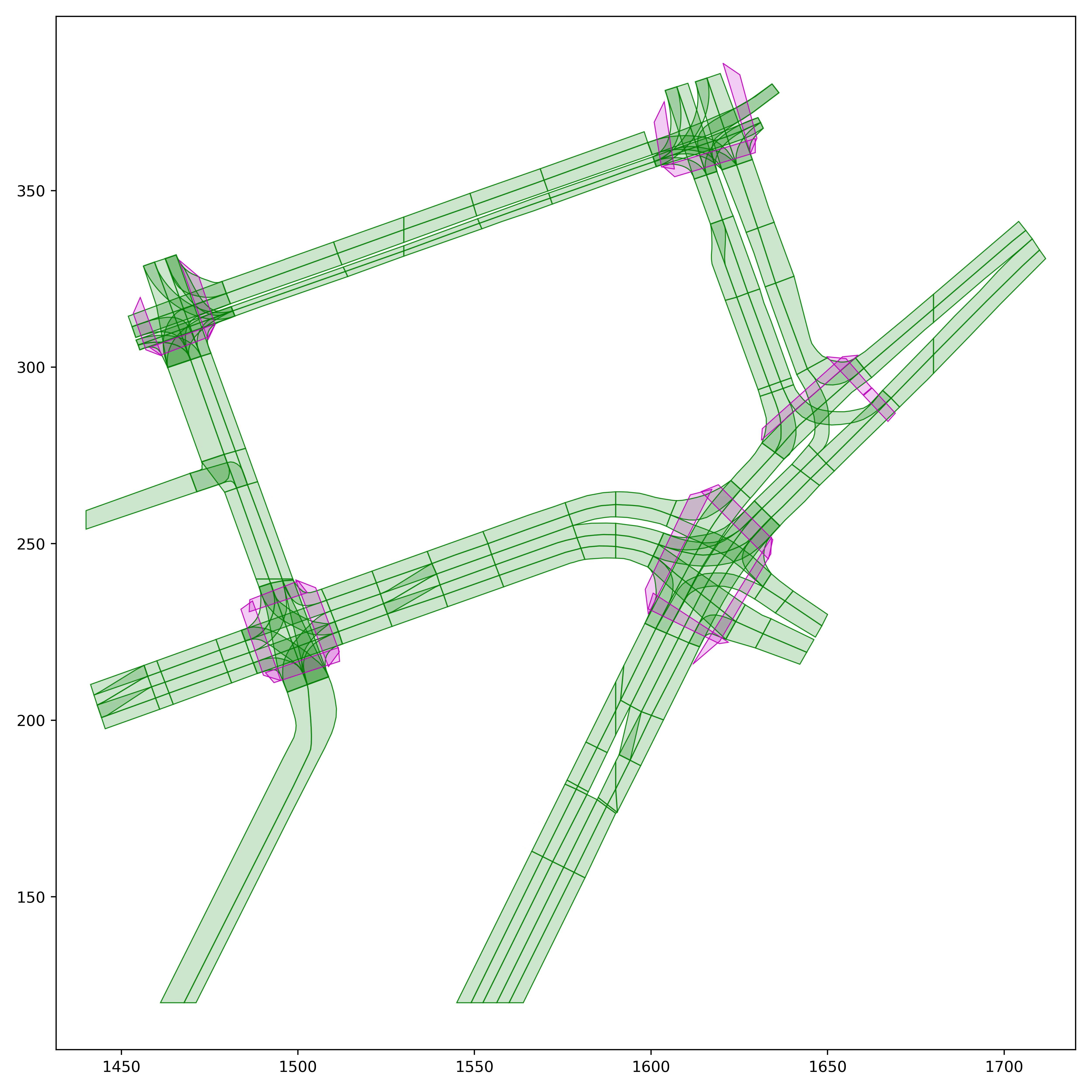
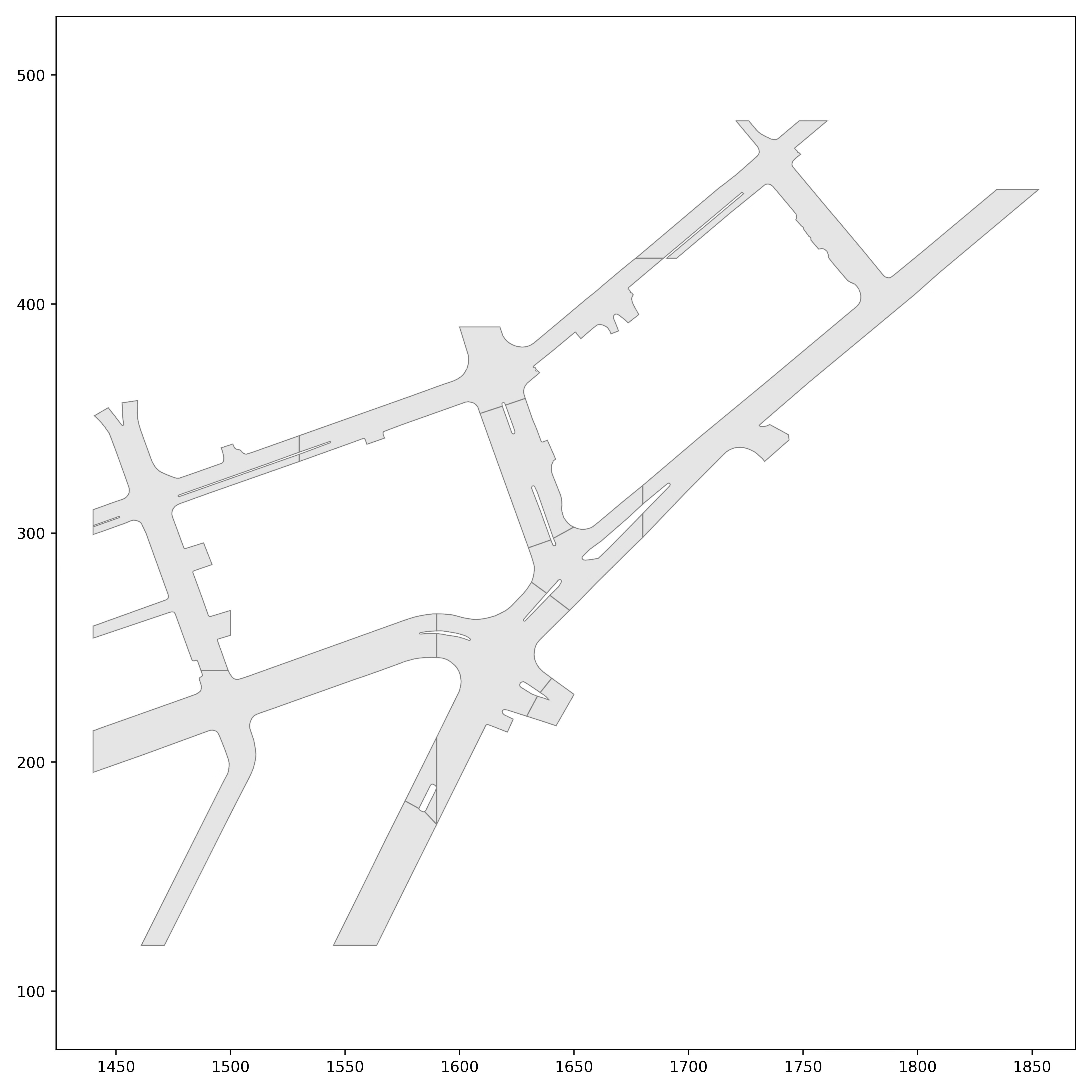
Table of Contents
- Overview
- Map Counts
- Vector Map: Lane Graph and Lane Segments
- Vector Map: Drivable Area
- Vector Map: Pedestrian Crossings
- Area of Local Maps
- Raster Maps: Ground Surface Height
- Training Online Map Inference Models
Overview
In all three datasets, each scenario contains its own HD Map with 3D lane, crosswalk, and drivable area geometry — sourced from data captured in six distinct cities (Austin, Detroit, Miami, Palo Alto, Pittsburgh, and Washington D.C.).
Each scenario in the three datasets described above shares the same HD map representation. Each scenario carries its own local map region. This is a departure from the original Argoverse datasets in which all scenarios were localized onto two city-scale maps. Advantages of per-scenario maps include:
- More efficient queries.
- The ability to handle map changes. A particular intersection might be observed multiple times in our datasets, and there could be changes to the lanes, crosswalks, or even ground height in between the times when the logs or sequences were captured.
Map Counts
Argoverse 2 offers a massive number of highly diverse HD maps:
- Motion Forecasting Dataset: ~250,000 vector maps.
- Sensor Dataset: 1,000 vector maps and 1,000 ground height raster maps.
- LiDAR Dataset: 20,000 vector maps.
- TbV Dataset: 1,038 vector maps and 1,038 ground height raster maps.
The core data structure that holds Argoverse 2 map data is the ArgoverseStaticMap class. Please refer to the map tutorial notebook for more examples of how to use the map API.
Vector Map: Lane Graph and Lane Segments
The core feature of the HD map is the lane graph, consisting of a graph , where are individual lane segments. In the supplemental material, we enumerate and define the attributes we provide for each lane segment. Unlike Argoverse 1, we provide the actual 3D lane boundaries, instead of only centerlines. However, our API provides code to quickly infer the centerlines at any desired sampling resolution. Polylines are quantized to resolution in the release.

These vector map files are provided as JSON, e.g. log_map_archive_00a6ffc1-6ce9-3bc3-a060-6006e9893a1a____PIT_city_31785.json
They may be loaded as follows:
from av2.map.map_api import ArgoverseStaticMap
log_map_dirpath = Path("av2") / "00a6ffc1-6ce9-3bc3-a060-6006e9893a1a" / "map"
avm = ArgoverseStaticMap.from_map_dir(log_map_dirpath=log_map_dirpath, build_raster=False)
Please refer to the LaneSegment class, with the following attributes:
id: unique identifier for this lane segment (guaranteed to be unique only within this local map).is_intersection: boolean value representing whether or not this lane segment lies within an intersection.lane_type: designation of which vehicle types may legally utilize this lane for travel (seeLaneType).right_lane_boundary: 3D polyline representing the right lane boundary (seePolyline).left_lane_boundary: 3D polyline representing the left lane boundary.right_mark_type: type of painted marking found along the right lane boundary (seeLaneMarkType).left_mark_type: type of painted marking found along the left lane boundary.predecessors: unique identifiers of lane segments that are predecessors of this object.successors: unique identifiers of lane segments that represent successor of this object. Note: this list will be empty if no successors exist.right_neighbor_id: unique identifier of the lane segment representing this object’s right neighbor.left_neighbor_id: unique identifier of the lane segment representing this object’s left neighbor.
Vector Map: Drivable Area
Instead of providing drivable area segmentation in a rasterized format, as we did in Argoverse 1, we release it in a vector format (i.e. as 3D polygons). This offers multiple advantages, chiefly in compression - allowing us to store separate maps for tens of thousands of scenarios, while ensuring that the raster format is still easily derivable. The polygon vertices are quantized to 1 cm resolution.
Please refer to the DrivableArea class, with the following attributes:
id: unique identifier.area_boundary: 3D vertices of polygon, representing the drivable area’s boundary.
Vector Map: Pedestrian Crossings
These entities represent crosswalks, and are provided in vector format. They are parameterized by two edges along a principal axis. Both lines should be pointing in nominally the same direction and a pedestrian is expected to move either roughly parallel to both lines or anti-parallel to both lines.
Please refer to the PedestrianCrossing class, with the following attributes:
id: unique identifier of pedestrian crossing.edge1: 3D polyline representing one edge of the crosswalk, with 2 waypoints.edge2: 3D polyline representing the other edge of the crosswalk, with 2 waypoints.
Area of Local Maps
Each scenario’s local map includes all entities found within a dilation in -norm from the ego-vehicle trajectory.
Raster Maps: Ground Surface Height
Only the AV2 Sensor Dataset and TbV includes a dense ground surface height map. (The AV2 LiDAR dataset and AV2 Motion Forecasting (MF) datasets do not come up with raster maps, but still have sparse 3D height information on polylines).
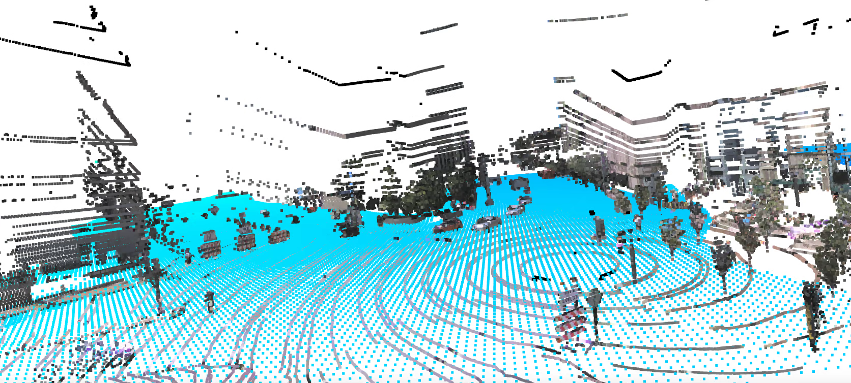
Ground surface height is provided for areas within a 5 m isocontour of the drivable area boundary, which we define as the region of interest (ROI). We do so because the notion of ground surface height is ill-defined for the interior of buildings and interior of densely constructed city blocks, areas where ground vehicles cannot observe due to occlusion. The raster grid is quantized to a 30 cm resolution, a higher resolution than the 1 m resolution in Argoverse 1.
This data is provided as float16 Numpy files:
00a6ffc1-6ce9-3bc3-a060-6006e9893a1a_ground_height_surface____PIT.npy
Sim(2) representation: In order to access the raster values, a Similarity(2) mapping from city coordinates to the high-resolution raster grid (which we refer to as img or array). This Similarity(2) object provided as a JSON file per log encapsulating (R,t,s), e.g.:
00a6ffc1-6ce9-3bc3-a060-6006e9893a1a___img_Sim2_city.json
Points may be transformed as follows:
from av2.geometry.sim2 import Sim2
array_Sim2_city = Sim2.from_json(json_fpath)
points_array = array_Sim2_city.transform_from(points_city)
However, instead of indexing manually into the raster arrays, the API will handle this for you:
avm = ArgoverseStaticMap.from_map_dir(log_map_dirpath=log_map_dirpath, build_raster=True)
points_z = avm.raster_ground_height_layer.get_ground_height_at_xy(points_xy)
Training Online Map Inference Models
Argoverse 2 offers new opportunities for training online map inference models, as the largest source of paired sensor data and HD maps publicly available at the time of release.
However, a few Sensor Dataset logs intentionally feature HD map changes:
75e8adad-50a6-3245-8726-5e612db3d16554bc6dbc-ebfb-3fba-b5b3-57f88b4b79caaf170aac-8465-3d7b-82c5-64147e94af7d6e106cf8-f6dd-38f6-89c8-9be7a71e7275
These logs should not be used for training online map inference models, as the real-world scene has recently been updated via constructed, leaving the map out-of-date.
Supporting Publications
Please use the following citation when referencing the Argoverse 2 Sensor, Lidar, or Motion Forecasting Datasets:
@INPROCEEDINGS { Argoverse2,
  author = {Benjamin Wilson and William Qi and Tanmay Agarwal and John Lambert and Jagjeet Singh and Siddhesh Khandelwal and Bowen Pan and Ratnesh Kumar and Andrew Hartnett and Jhony Kaesemodel Pontes and Deva Ramanan and Peter Carr and James Hays},
  title = {Argoverse 2: Next Generation Datasets for Self-Driving Perception and Forecasting},
  booktitle = {Proceedings of the Neural Information Processing Systems Track on Datasets and Benchmarks (NeurIPS Datasets and Benchmarks 2021)},
  year = {2021}
}
Use the following citation when referencing the Trust, but Verify Map Change Detection Dataset:
@INPROCEEDINGS { TrustButVerify,
  author = {John Lambert and James Hays},
  title = {Trust, but Verify: Cross-Modality Fusion for HD Map Change Detection},
  booktitle = {Proceedings of the Neural Information Processing Systems Track on Datasets and Benchmarks (NeurIPS Datasets and Benchmarks 2021)},
  year = {2021}
}
We value your feedback. If you have any comments, suggestions, or issues please reach out to us on Github.
Contributing
Have a cool feature you’d like to add? Found an unhandled corner case? The Argoverse team welcomes contributions from the open source community - please open a PR using the following template!
Terms and Conditions
Table of Contents
Licensing
By using or downloading Argoverse, you are agreeing to comply with the terms of this page and any licensing terms referenced below.
License - Data and Documentation. Argoverse and any associated data or documentation are provided free of charge under the terms of the Creative Commons Attribution-NonCommercial-ShareAlike 4.0 International Public License (“CC BY-NC-SA 4.0”). The full text of the license is accessible at https://creativecommons.org/licenses/by-nc-sa/4.0/legalcode.
License - Code and Documentation. Argoverse code and APIs are licensed under the MIT license, the full text of which can be found at https://opensource.org/licenses/MIT.
Using the Argoverse Non-Commercially. We license Argoverse data and documents for non-commercial use only. Under the terms of the CC BY-NC-SA 4.0 “non-commercial” means “not primarily intended for or directed towards commercial advantage or monetary compensation.”
Suggestions. If you use Argoverse and identify areas that could benefit from changes, we would like to hear from you. Please submit any comments on the issues page of our GitHub repository. If you submit your changes, you may be required to confirm that your changes are subject to CC BY-NC-SA 4.0.
Attribution. Please follow the attribution guidelines provided in section 3.A. of CC-BY-NC-SA 4.0 license with the copyright notice being “© 2018-2022 Argo AI, LLC”. APIs attribution shall comply with the MIT license.
Privacy. Argoverse takes steps to protect the privacy of individuals by blurring faces and license plates. If you notice that your face or license plate is still identifiable, or if you have any privacy concerns pertaining to Argoverse, please contact us.
Competitions
NO PURCHASE OR PAYMENT OF ANY KIND NECESSARY. A PURCHASE OR PAYMENT OF ANY KIND WILL NOT INCREASE YOUR CHANCES OF WINNING. THIS COMPETITION IS VOID WHERE PROHIBITED. BY ENTERING THIS COMPETITION, EACH ENTRANT AGREES TO THE FOLLOWING TERMS AND CONDITIONS.
Eligibility. The CVPR 2023 competition is open to currently enrolled university students, university faculty members, and other individuals who are 18 years of age or older at the time of entry. Eligible entrants can participate in the competition as an individual or as a team.
Competition Period. All entries submitted from May 1, 2022 through the end of the competition at 11:59PM EST on June 11th, 2023 (“Competition Submission Period”) will be considered. Entries submitted before or after the Competition Submission Period will not be considered or eligible to win.
How to Enter. To enter the competition, eligible entrants must (1) Create an account at https://evalai.cloudcv.org/ (the “Website”); (2) Access and use the Argoverse data test sets available through https://www.argoverse.org to produce the predictions our outputs relevant to each competition (e.g. motion forecasts, scene flow estimations, occupancy predictions, etc); (3) Submit files containing their predictions through the Website before the end of the Competition Submission Period; and (4) Submit a one page or longer report to argoverse-competition@argo.ai describing the algorithms used in the entry before the end of the Competition Submission Period. This report will be used for determining which works are highlighted at CVPR.
Personal Data. While signing up to enter the competition, an entrant will be asked to provide personal information including the entrant’s name and email address. Sponsor may use this information to contact entrants about their competition entries, and with newsletters, marketing or promotional materials and other information that may be of interest to entrants. Entrants may (i) opt out of, or (ii) withdraw his or her consent from, receiving any or all of these communications from Sponsor (unless required to provide the competition to the entrant) by following the unsubscribe link located in the footer of any email received from Sponsor. Please refer also to Sponsor’s Privacy Policy.
Limit per Individual/Team. A maximum of 2 submissions per day and a maximum of 100 submissions in total. We will disqualify teams that use proxy accounts to get around this limit.
Selection and Notification of Winners. Beginning on or about June 7th, 2024, entries will be judged based on the Evaluation Criteria posted on the Website. Winners will be notified on or after June 15th, 2023 by email, and will be announced at the Workshop on Autonomous Driving at the 2024 Conference on Computer Vision and Pattern Recognition (“CVPR 2024”) on June 17th, 2024. A winner will be disqualified and an alternate winner may be selected if a selected winner fails to comply with these terms and conditions; cannot be contacted; or is ineligible.
By entering this competition, each entrant agrees that his or her biographical information, and other content provided by entrant and members of his or her team, may be publicly announced and posted in connection with the competition, including, without limitation, through posting online. An entrant can withdraw his or her consent at any time for the future. An entrant’s withdrawal of consent shall not affect the lawfulness of processing based on consent before the withdrawal. Where an entrant provides information or content of his or her team members, the entrant warrants that the respective individuals have consented to the publication of such information as described above.
All decisions of Sponsor regarding the selection of winners, notification, and substitution of winners in accordance with these terms and conditions shall be binding and final. Winners will be determined as specifically described above, and not using any random drawing or method incorporating chance.
Prize Details
There are no prizes. However, winners will be highlighted at the Workshop on Autonomous driving and on the Argoverse web page.
Copyright and Moral Rights. By entering this competition, entrants warrant to Sponsor that they created their competition entries, that they own all of the copyright interests in the materials submitted in connection with those entries, and that Sponsor’s use of such entry materials in accordance with these terms and conditions will not infringe any person’s intellectual property rights or other legal rights. Further, by entering this competition, entrants grant Sponsor an exclusive, worldwide, royalty-free, perpetual and irrevocable license to copy, store, modify, transmit, use, and publish all entry materials including algorithms, predictions, and other components of their competition entries.
Disqualification/Termination/Modification of the Competition. Individuals who tamper with or abuse any aspect of this competition or the Website, as solely determined by Sponsor, will be disqualified. If for any reason this competition is not capable of running as planned due to infection by computer virus, bugs, tampering, unauthorized intervention, fraud, technical failures, or any other causes beyond the control of Sponsor which corrupt or affect the administration, security, fairness, integrity, or proper conduct of this competition, Sponsor reserves the right at its sole discretion, to cancel, terminate, modify, or suspend the competition, in whole or in part, at any time, without notice. Should any such action be taken, Sponsor may determine a winner from valid, non-suspect entries received prior to action taken, or otherwise as deemed fair and equitable by Sponsor.
Limitations of Liability and Release. Sponsor is not responsible for lost, late, misdirected or undelivered entries, or for lost, interrupted or unavailable satellite, network, server, Internet Service Provider (ISP), Website, or other connections availability, accessibility or traffic congestion, miscommunications, failed computer, network, telephone, satellite or cable hardware or software or lines, or other errors of any kind whether human, mechanical, electronic or network. Further, to the greatest extent permitted by applicable law, Sponsor is not responsible for any injury or damage to entrants or any other person’s computer or property related to or resulting from participation in this competition.
By entering the competition, to the extent permitted by applicable law, each entrant agrees to release and hold Sponsor, its affiliates, subsidiaries, parent companies, officers, directors, employees, agents, and any other companies participating in the design, administration or fulfillment of this competition and their respective officers, directors, employees, and agents, harmless from any and all losses, rights, claims, injuries, damages, expenses, costs or actions of any kind resulting in whole or in part, directly or indirectly, from entrant’s participation in this competition, including any such matters arising from any competition-related activity, including but not limited to, selection of winners.